Generate random numbers in MS Excel

A common requirement is to generate a set of random numbers that meet some underlying criterion. For example, a set of numbers that are uniformly distributed from 1 to 100. Alternatively, one might want random numbers from some other distribution such as a standard normal distribution.

While there are specialized algorithms to generate random numbers from specific distributions, a common approach relies on generating uniform random numbers and then using the inverse function of the desired distribution. For example, to generate a random number from a standard normal distribution, use =NORM.S.INV(RAND())

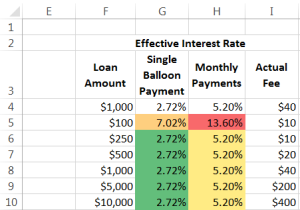
Another common requirement is the generation of integer random numbers from a uniform distribution. This might be to select people for something like, say, training, or a drug test. Or, it might be to pick a winner for a door prize at a social event. It might also be to assign players to groups for a sport tournament such as golf.

For a version in a page by itself (i.e., not in a scrollable iframe as below) visit http://www.tushar-mehta.com/publish_train/xl_vba_cases/0806%20generate%20random%20numbers.shtml

Tushar Mehta

Draw a circle in an Excel chart

By default, Excel has a limited number of charts. That does not mean that those are the only charts one can create. It turns out that with a little imagination and creativity, we can format and configure the default charts so that the effect is like many other kinds of charts.

One of the more versatile of charts is the XY Scatter chart. We can use it as the base for many data visualization tasks. Recently, for a client, I used one to create a radial org chart as in Figure 1. Such a chart is also called a Node-Link chart or a Reingold–Tilford Tree.

image001
Figure 1 – Example of a radial org graph created in an Excel XY Scatter chart
after removal of all identifiable information and the obfuscation of data
necessary to protect the client’s confidentiality.

A lot of “out of the box” work into making this chart. One key element was the set of equidistant concentric circles that provide a visual reference for the small colored dots. This note demonstrates how to create concentric circles in an Excel XY Scatter chart.

For a version in a page by itself (i.e., not in a scrollable iframe as below) visit http://www.tushar-mehta.com/publish_train/xl_vba_cases/0610%20draw%20circle.shtml

Tushar Mehta

Analyze ‘free’ money

Recently, I received yet another promotion from yet another company offering me money at zero percent interest with the predictable asterisk next to the zero percent. Instead of just shredding the offer I decided to create a downloadable Excel template to analyze the offer, which was an interest-free 18 month loan for a 4% transaction fee with a minimum $10 fee.

Obviously, the transaction fee makes sure that the money is not ‘free.’ So, how does one calculate the cost of even the best emergency loans? I settled on an “effective interest rate.”

image001

For a version in a page by itself (i.e., not in a scrollable iframe as below) visit http://www.tushar-mehta.com/publish_train/xl_vba_cases/0920%20free%20money.shtml

Tushar Mehta

Excel corrupts certain workbooks in migrating from 2003 to 2007

I got a email from a client asking for help because Excel was “destroying,” to use his terminology, his 2003 workbook after conversion to the 2007 format. And, after analyzing the kind of change Excel made, I had to agree.

The following in 2003

badnames 1
Figure 1

becomes, in 2013 (and in 2010),

badnames 5
Figure 2

The basic problem is that names that are legitimate names in Excel 2003 may become unacceptable in 2007 (or later). But, a more devastating problem is with a formula using a name with a dot in it. Even though it is completely legitimate, Excel changes the dot to a colon. This causes the formula =SW1.SW2 to become =SW1:SW2. Don’t ask me why. It just does. The result is the formula is all wrong and destroys the integrity of the workbook.

It appears that the cause may be Excel trying to help manage the transition of a XLS workbook into the newer format. In 2007, Microsoft increased the number of columns from 256 to 16,384. Consequently, the reference to last column went from IV to XFD. So, a name such as SW1, completely OK in 2003, became unacceptable in 2007. On converting a XLS file to a XLSX file, Excel will convert such names by adding an underscore at the start of the name. But, it seems to go beyond that, converting formula references to certain names with dots in them to a colon. This happens if both the tokens to the left and to the right of the dot could be legitimate cell references. So, Excel converts the formula =XFD1.XFD2 to =XFD1:XFD2 but it will leave =XFD1.XFE2 alone.

To replicate the problem:

  • Start with Excel 2003. Create a workbook and add the names shown in the Figure 1. Save and close the workbook.
  • Open the workbook in Excel 2013. Save it as a XLSX file. Acknowledge the warning message (see Figure 3),

    badnames 3
    Figure 3

  • Close and reopen the new XLSX workbook. The formulas will have the errors shown in Figure 2.

The safest way to work around this problem is to add an underscore before every name in the workbook before making the transition to the 2007 format. Obviously, the quickest way to do this would be with a very simple VBA procedure. But, through trial and error I discovered the code will not work in 2003. It runs without any problems but it doesn’t do anything!

So, the correct way to use the code is the following sequence.

  • Open the XLS file in 2013 (or 2010).
  • Run the macro below.
  • Now, save the file in the newer format. If your original workbook had no code in it, save the file as a XLSX file and acknowledge the warning that the VB project will be lost.
  • Close and reopen the file. You should see the correct data with all the names now starting with an underscore.

    badnames 7
    Figure 4

Tushar Mehta

RIP Live Mesh, hello Cubby

Recently, I have had to make changes to my “computing infrastructure.” This is one of them.

blog-Picture1
blog-Live_Mesh_Logo
blog-Cubby-Logo

For the longest time I synchronized files between my laptop and desktop with the help of a flash drive.

Then, I discovered Groove but it didn’t really fit the bill and I don’t remember why.

It was on to FolderShare at about the same time that it became a free product. And, it worked wonderfully.

What was really neat about it was that it synced folders peer-to-peer. The files were not on a server and if both computers were on the same LAN, they didn’t even touch the ‘Net!

Microsoft acquired it and it still worked. It became Live Sync and I dreaded each new version but luckily it continued to work. Though, I noticed there were serious lags in file sync. From what I could tell — and I could be wrong — the server played a critical role in deciding which files needed syncing and that introduced a bottleneck. Live Sync became Windows Live Mesh and at some point it included a cloud-based sync capability, which I never used.

This peer-to-peer sync model fit in very well when I got married and my wife delegated all “computer support” to me. So, I extended Live Sync to her computers, duplicated her files on my computer and and included her files in my backups.

Earlier this year, in Feb. 2013, Microsoft discontinued Live Sync, which by now was named Live Mesh. In researching alternatives, I narrowed the field to GoodSync and Cubby, the only two that supported peer-to-peer sync. GoodSync was priced per computer: $30/Windows and $40/Mac; Cubby works on a subscription: $84/year. Given the proliferation of devices, Cubby made more sense.

The interesting thing about Cubby is that it has a free version that includes 5GB of cloud storage but no peer-to-peer capability. Upgrade to Pro (that’s the $84/year subscription), and it includes 100GB of cloud storage. Of course, with the peer-to-peer DirectSync, I don’t care about the expanded cloud storage. Cubby has other features that I haven’t explored yet including customer specified encryption keys.

Worksheet as a chart – multiple conditional formats

Several years back, I wrote an article on how to use multiple cells to simulate conditional formats that involved more than 3 conditions. Three versions of Excel later, I still receive requests related to this post. So, I updated it to include more screenshots and a downloadable file.

In Excel 2003 and earlier, conditional formatting works well for up to three conditions. But even when the number of conditions exceeds that limit, it is possible to do without any programming support. For example, one possible way to show twelve possible rankings through color is shown below.

img7img8img9

For more see http://www.tushar-mehta.com/excel/newsgroups/worksheet_as_chart/

Tushar Mehta

TM Goal Seek

TM Goal Seek enhances the existing user interface to Excel’s Goal Seek feature. The built in Goal Seek is a simple optimization tool that suffices for a large number of scenarios. The UI, unfortunately, is extremely unwieldy and unfriendly. TM Goal Seek is a simple add-in that is easier to use than the default dialog box because of three critical benefits:

  1. The target value can be a number or a reference to a cell that contains a number,
  2. The add-in retains values previously entered in the dialog box, and
  3. One can interact with the worksheet even with the dialog box open.

The motivation to develop the add-in came from work I was doing for a client who managed gambling sites not on gamstop that involved risk analysis on multiple investment scenarios of financial derivative trades. The default Goal Seek interface took way too long.

The current version of the add-in will expire on May 1, 2013.

For more see http://www.tushar-mehta.com/excel/software/goal_seek/index.htm

Tushar Mehta