Worksheet as a chart – multiple conditional formats

Several years back, I wrote an article on how to use multiple cells to simulate conditional formats that involved more than 3 conditions. Three versions of Excel later, I still receive requests related to this post. So, I updated it to include more screenshots and a downloadable file.

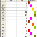
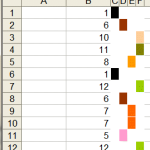
In Excel 2003 and earlier, conditional formatting works well for up to three conditions. But even when the number of conditions exceeds that limit, it is possible to do without any programming support. For example, one possible way to show twelve possible rankings through color is shown below.

img7img8img9

For more see http://www.tushar-mehta.com/excel/newsgroups/worksheet_as_chart/

Tushar Mehta

Highlight row and column of active cell

By default, when the user selects a cell, Excel highlights the row and column by changing the color of the associated row and column headers. This tip shares multiple ways to highlight the row and column in more obvious ways as well as a way to highlight the cell in a specific column in the same row.


The emphasis is on the use of conditional formatting to accomplish the task. The minimal VBA code required to make it work is the same single executable statement for all of the different highlighting options!

For a version in a page by itself (i.e., not in a scrollable iframe as below) visit http://www.tushar-mehta.com/publish_train/xl_vba_cases/0121%20highlight%20row%20and%20col%20of%20selected%20cell.shtml

Tushar Mehta