It’s Evil Function election time: cast your votes so we can find out what the most evil Excel function is!
My vote has gone to INDIRECT (see my blog post here)
I will publish the results when we have got enough votes.
It’s Evil Function election time: cast your votes so we can find out what the most evil Excel function is!
My vote has gone to INDIRECT (see my blog post here)
I will publish the results when we have got enough votes.
Everyone knows that SUBTOTAL ignores filtered rows. Readers of DDoE know that SUBTOTAL also ignores other SUBTOTAL formulas. I tell everyone who will listen about the benefits of SUBTOTAL. It’s one of the best received tips in the ‘Tips and Tricks’ portion of the training I do. But I still get spreadsheets that use SUM and individual adding of cells. When I do, I convert them to SUBTOTAL to make sure there are no errors. Today, I decided to automate that process.
I’ve filled column B over to the right into column C so I can preserve the original data.
With Excel’s color coding and this simple worksheet, you may have spotted the error in the grand total formula. Below is the code I wrote to correct this situation without having to put in all the SUBTOTALs manually.
|
1 2 3 4 5 6 7 8 9 10 11 12 13 14 15 16 17 18 19 20 21 22 23 24 25 26 27 28 |
Public Sub ConvertSumToSubtotal() Dim rCell As Range Dim rStart As Range Const sSUM As String = "=SUM(" 'Only work on ranges If TypeName(Selection) = "Range" Then 'Only work on single columns If Selection.Columns.Count = 1 Then 'rStart will adjust to be where ever the SUBTOTAL range will start Set rStart = Selection.Cells(1) 'loop through the cells and replace SUM with SUBTOTAL 'change rStart to point to cell just below the SUBTOTAL For Each rCell In Selection.Cells If rCell.HasFormula And Left(rCell.Formula, 5) = sSUM Then rCell.Formula = "=SUBTOTAL(9," & rStart.Address(0, 0) & ":" & rCell.Offset(-1, 0).Address(0, 0) & ")" Set rStart = rCell.Offset(1, 0) End If Next rCell End If End If 'Make the last cell a SUBTOTAL of the whole range Selection.Cells(Selection.Rows.Count).Formula = "=SUBTOTAL(9," & Selection.Resize(Selection.Rows.Count - 1, 1).Address(0, 0) & ")" End Sub |
This won’t work in every situation, but this layout is the one I see the most. This layout being SUMs for the subtotals and a big =A1+A2+A3 style formula for the grand total.
Once again SUBTOTAL saves the day and fixes the error. The most common error I see with this layout is in the grand total, but not always. Sometimes the subtotals don’t cover the correct range. It would seem easier when replacing the SUMs to use the same range the SUM uses, but I wanted to make sure I fixed any of those errors too. To do that, I SUBTOTAL from the cell below the previous SUBTOTAL to the cell above the current one.
Pro tip: Use
|
1 |
Ctrl+` |
to toggle between viewing formulas and values (that’s an accent grave, left of the 1 key on US keyboards).
A reader needs to find the difference between the time listed and the earliest time listed for that same day. Here’s the data:
| Date | Time | Difference |
|---|---|---|
| 6/9/2014 | 14:49:05 | 0:00:00 |
| 6/9/2014 | 14:49:47 | 0:00:42 |
| 6/9/2014 | 14:50:33 | 0:01:28 |
| 6/9/2014 | 14:51:17 | 0:02:12 |
| 6/9/2014 | 14:51:31 | 0:02:26 |
| 6/9/2014 | 14:51:56 | 0:02:51 |
| 7/9/2014 | 6:19:55 | 0:00:00 |
| 7/9/2014 | 6:21:09 | 0:01:14 |
| 7/9/2014 | 6:21:31 | 0:01:36 |
| 7/9/2014 | 6:22:25 | 0:02:30 |
| 7/9/2014 | 6:22:53 | 0:02:58 |
| 7/9/2014 | 6:23:23 | 0:03:28 |
| 7/9/2014 | 6:23:47 | 0:03:52 |
The formula in the Difference column, C2, is
|
1 |
{=B2-MIN(IF($A$2:$A$14=A2,$B$2:$B$14,""))} |
, filled down to fit the data.
It’s an array formula, so don’t type the curly braces, but enter with Ctrl+Shift+Enter, not just enter. The array part of the formula, the part subtracted from B2, is the smallest value where the date in column A is a match. By selecting everything in the MIN function in the formula bar and pressing Ctrl+=, you can see how Excel is calculating the minimum.
|
1 |
=B2-MIN({0.617418981481482;0.617905092592593;0.6184375;0.618946759259259;0.619108796296296;0.619398148148148;"";"";"";"";"";"";""}) |
Because we’re dealing with times, the numbers aren’t so easy to read. But the important part is at the end of the array – a bunch of empty strings. When the date doesn’t match, the IF function returns an empty string. MIN ignores any text, so only the smallest of the numbers listed is returned.
It’s fun to argue about whether VLOOKUP or INDEX/MATCH is better, but to me that’s missing the point: they are both bad.
So I decided to design and build some better ones.
Here are some of the more-frequently mentioned VLOOKUP INDEX/MATCH problems
MEMLOOKUP ( Lookup_Value, Lookup_Array, Result_Col, Sort_Type, MemType_Name, Vertical_Horizontal )
The syntax is designed to make it easy to convert a VLOOKUP to MEMLOOKUP, but there are differences!
It’s always tempting to cram in more function (scope creep is universal), but if the result is too many parameters then it’s a mistake. So instead there is a whole family of these lookup functions that build on the MEMLOOKUP/MEMMATCH technology to provide the ultimate in flexibility and power whilst remaining efficient.
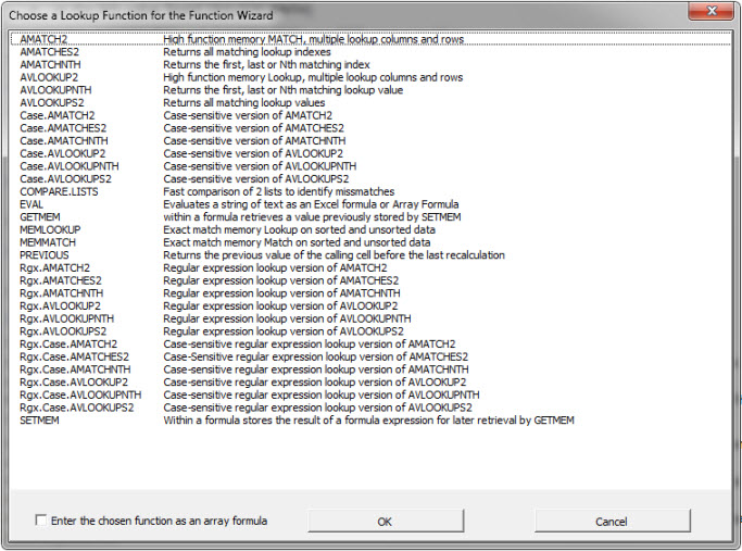
These functions are included in the 90 or so additional Excel functions built into FastExcel V3.
You can download the trial version from here.
I would be delighted to tell the Excel team how I built these functions and the algorithms they use.
By the way they are written as C++ multi-threaded functions in an XLL addin for maximum performance.
On this episode of the BBC’s More or Less podcast, they discussed big, round birthdays that fall on a weekend. A listener said that she had to wait until her 60th birthday for it to fall on a weekend. The guy who figured out how unlucky she was tested every birthday from January 1, 1900. Since he picked that date, I assume he used Excel, but he never said.
They did include the caveat “as an adult” so that leaves off the 10th birthday. Here’s how I did the math.
I started with 1/1/1900 is cell A2 and used the formula
=A2+1
copied down to today. Then in B1:J1, I entered the values 20-100. The formula in B2 is
=WEEKDAY(DATE(YEAR($A2)+B$1,MONTH($A2),DAY($A2)),2)>=6
I added the value in row 1 to the year to make the centennial birthday and fed that into the WEEKDAY function. WEEKDAY returns 1 through 7 representing the day of the week. I used ‘2’ for the second argument so that Monday is 1 and Saturday is 6. Then I return TRUE or FALSE depending on whether the weekday is greater than or equal to 6.
Column K finds the minimum age that has a TRUE under it
=MIN(IF(B2:J2,$B$1:$J$1,""))
That’s an array formula, so I entered it with Ctrl+Shift+Enter.
Next, I repeated 20-100 in column N. These formulas complete the table
    O3        =COUNTIF($K$2:$K$41832,N3)

    P3        =O3/SUM($O$3:$O$11)

    Q3        =Q2+P3
As if that wasn’t enough, I wanted to make a single formula that could accept a date and return the earliest major birthday that was on a weekend.
=MIN(IF(WEEKDAY(DATE(YEAR(O16)+{20,30,40,50,60},MONTH(O16),DAY(O16)),2)<6,"",{20,30,40,50,60}))
That's also an array formula, so you know what to do. I celebrated my 30th birthday on a weekend.
I was writing some formulas for a tiered commission calculation recently that I thought I should post. But beyond just what the formulas do, it reminded me that I’ve never shared my ‘counting zeros’ opinion, so I’m wrapping that in with this post too.
You have a commission structure where you pay your salesmen 5% for every sale. If the sale is a particularly large one, you pay them a bonus commission – 8% for the portion of the sale that’s over $20,000. But you don’t want your salespeople getting so rich that they have enough money to quit. Nor do you want them to get an unfairly huge commission on an unusually large sale. So you have a third tier that reduces their commission to 1% for the portion of the sale that’s over $100,000.
Let’s look at the formulas for column H.
    H4        =MAX(MIN(2*10^4,H2)*0.05,0)

    H5        =MAX(MIN(8*10^4,H2-2*10^4)*0.08,0)

    H6        =MAX(0,H2-10^5)*0.01
The MIN part of the formulas in H4 and H5 make sure you don’t pay more commission on that tier than you should. The MAX part returns zero when the calculation goes negative.
About counting zeros. You may have noticed that I use terms like 2*10^4 to represent $20,000. I’m a big fan of commas, but I can’t use them in formulas (they’re kind of important for separating arguments). I picked up using scientific notation in formulas from a scientist I know and I love it. No more do I have count the zeros in
=IF(A1=25000000,600000,8000000)
to know if it’s 25 million, 2.5 million, or 250 million. Instead I write
=IF(A1=25*10^6, 6*10^5, 8*10^6)
An even better answer is to put those values in cells and refer to the cells. When they’re in cells, I can format them and use commas to count the zeros. But let’s face it, sometimes we hardcode numbers in formulas. And when I do, I’ve been using this method for larger numbers and, after a small adjustment period, it’s been great.
Sometimes I just want to quickly see the difference between two cells or groups of cells. Excel puts some great aggregates in the status bar.
and you can even customize them. Right click on the those aggregates.
But I wanted the difference. So I wrote some code to find it. I already had a class module with an Application object declared WithEvents, so I added this SheetSelectionChange event procedure.
|
1 2 3 4 5 6 7 |
Private Sub mxlApp_SheetSelectionChange(ByVal Sh As Object, ByVal Target As Range) If TypeName(Selection) = "Range" Then ShowDifferenceStatus Selection End If End Sub |
That event procedure calls this procedure in a standard module.
|
1 2 3 4 5 6 7 8 9 10 11 12 13 14 15 16 17 18 19 20 21 22 23 24 25 26 27 28 29 30 |
Public Sub ShowDifferenceStatus(rSel As Range) Dim wf As WorksheetFunction Dim vStatus As Variant On Error Resume Next Set wf = Application.WorksheetFunction If rSel.Areas.Count = 1 Then If rSel.Columns.Count = 2 Then vStatus = "Difference: " & Format(wf.Sum(rSel.Columns(1)) - wf.Sum(rSel.Columns(2)), "#,##0.00") ElseIf rSel.Rows.Count = 2 Then vStatus = "Difference: " & Format(wf.Sum(rSel.Rows(1)) - wf.Sum(rSel.Rows(2)), "#,##0.00") Else vStatus = False End If ElseIf rSel.Areas.Count = 2 Then If (rSel.Areas(1).Columns.Count = 1 And rSel.Areas(2).Columns.Count = 1) Or _ (rSel.Areas(1).Rows.Count = 1 And rSel.Areas(2).Rows.Count = 1) Then vStatus = "Difference: " & Format(wf.Sum(rSel.Areas(1)) - wf.Sum(rSel.Areas(2)), "#,##0.00") End If Else vStatus = False End If Application.StatusBar = vStatus End Sub |
If the selection is contiguous (Areas.Count = 1), it determines if there are two columns or two rows. Then it uses the SUM worksheet function to sum up the first and subtract the sum of the second. Anything other that two columns tow rows resets the StatusBar by setting it to False. Subtracting one cell from the other is easy enough, but I wanted the ability to subtract one column from the other (or one row). Using SUM also avoids me having to check for text or other nonsense that SUM does automatically. Here’s one where I only have one Area selected and it contains two columns. It sums the numbers in column B and subtracts the sum of column C.
When the selection is not contiguous (Areas.Count = 2), then it determines if both areas have only one column or only one row. If either has more than one, it resets the status bar. But if they both have one (of either), it subtracts them. Here I’ve selected B2:B3, then held down the Control key while I selected C3:C4. That’s two areas, but each only has one column, so it assumes I want to subtract columns.
The next feature I want to add is to recognize filtered data. Often I’m working with a filtered Table and although two cells appear to be adjacent, selecting them without holding down Control really selects all those filtered cells in between. I guess I’ll need to loop through and determine what’s visible, build a range from only those cells, and sum that. For now, I’m just holding down control and using the mouse to select them. If you’re not familiar, the “mouse” is that blob of plastic several inches away from home row (aka the productivity killer). Excuse me while I get off my soap box and finish this post.
I tried to glean the NumberFormat of the cells selected and use that in the display. You can see from the code above that I punted and just used a comma and two decimals. But that stinks for really small numbers. Originally, I had something like
|
1 |
vStatus = "Difference: " & Format(wf.Sum(rSel.Columns(1)) - wf.Sum(rSel.Columns(2)), rSel.Cells(1).NumberFormat) |
But look at the craziness when the cell as the Accounting format (_(* #,##0.00_);_(* (#,##0.00);_(* "-"??_);_(@_))
It works well for times though.
Apparently the syntax for cell formatting is slightly different than for the VBA.Format function. I haven’t worked out what the differences are, but maybe someday I will.
Hi all,
I’ve been working on my RefTreeAnalyser again. What I’ve been up to this time is building tools which help with the analysis of dependencies which are mostly hidden from view:
A new dialog has been added that shows all sources of the objects in your file:
Moreover, when you analyse a particular cell for its dependencies, objects are taken into account too (well, to be perfectly honest, only if you purchase a license):
If you haven’t already done so, why don’t you head over to my website and download the tool. The demo is free and (almost!) fully functional.
Regards,
Jan Karel Pieterse
www.jkp-ads.com