Matching Column Widths

Posted on July 1, 2016July 1, 2016 by Dick Kusleika

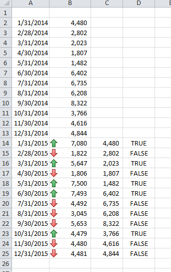
Here’s a report for a high volume, low margin product. Because the profit is so much smaller than sales and costs, column D is narrower than columns B and C.

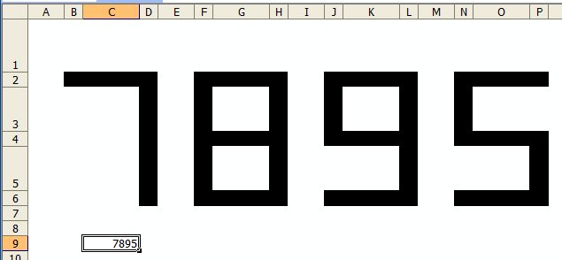
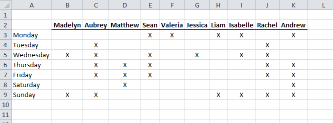
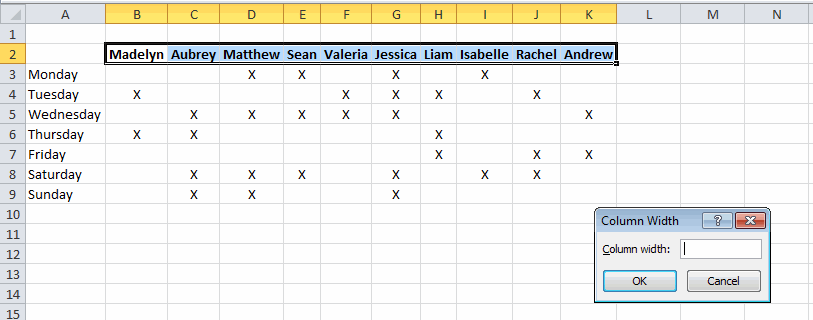
Another example is the following table with names across the top. When the column widths are set to autofit, they all become different widths. Of course that simply won’t do.

Drag Multiple Columns

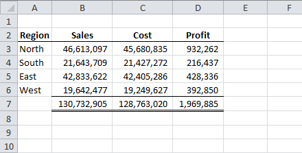
The first technique, and likely the most common, is to select all the columns and change the width of one of them. That will change the width of all of them. In the below figure, I select the entire columns B through K. It appears that column D is the largest so I select the column divider between D and E and drag it a few pixels to the right, then drag it back.

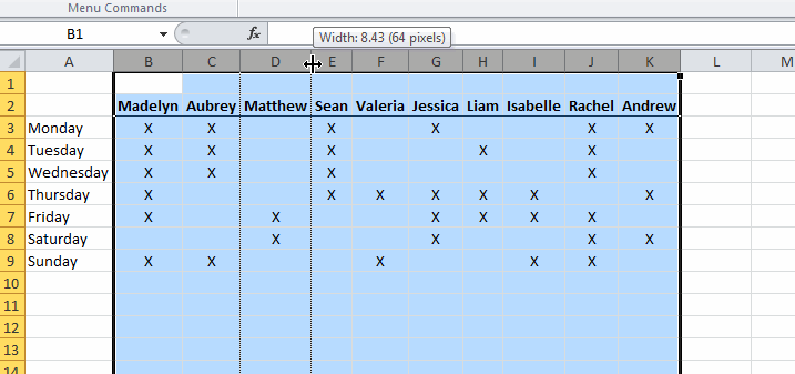
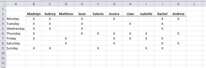
This changes all the selected columns to the width set for column D.

Well, that’s all I have to say about setting column widths. Of course I’m kidding. Let’s look at some keyboard only methods.

Format Column Widths

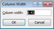
Select any cell in column D and click the Column Widths button on Home – Cells – Format (Alt + H + O + W). That will tell you the width of column D.

Make a note of the width and dismiss the dialog box (Esc). Now select cells in every column you want to change. For example, I selected B2:K2. It doesn’t have to be row 2. In fact, it could be multiple rows. All that matters is that every column that you want to change is included in the selection. Because the column widths aren’t the same, the Column Width dialog is empty.

I can type 8.43 in that box (the width of column D that I looked up earlier) and all the columns will be set to that width.

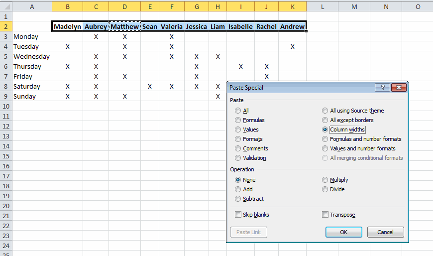
Paste Special

To use this method, select D2 and copy it (Ctrl+C). Next, select B2:K2 and choose Paste Special from the Ribbon (Alt + H + V + S). Choose the Column widths radio button (Alt+w) and click OK (Enter).

Build Your Own

You knew this was coming, didn’t you? Didn’t you? I wrote a macro and assigned it to Ctrl+Shift+W.

Public Sub MatchColumnWidths()
    
    Dim lMax As Double
    Dim rCell As Range
    
    gclsAppEvents.AddLog "^+w", "MatchColumnWidths"
    
    If TypeName(Selection) = "Range" Then
        If Selection.Cells.Count > 1 Then
            'if the first cell is active, set all columns to the biggest column
            If ActiveCell.Address = Selection.Cells(1).Address Then
                For Each rCell In Selection.Rows(1).Cells
                    If rCell.ColumnWidth > lMax Then lMax = rCell.ColumnWidth
                Next rCell
                For Each rCell In Selection.Rows(1).Cells
                    rCell.EntireColumn.ColumnWidth = lMax
                Next rCell
            'if the user selected a particular cell (not the first one), set
            'all columns to the selected column
            Else
                For Each rCell In Selection.Rows(1).Cells
                    rCell.EntireColumn.ColumnWidth = ActiveCell.ColumnWidth
                Next rCell
            End If
        End If
    End If
    
End Sub

Public Sub MatchColumnWidths()

Dim lMax As Double

Dim rCell As Range

gclsAppEvents.AddLog "^+w", "MatchColumnWidths"

If TypeName(Selection) = "Range" Then

If Selection.Cells.Count > 1 Then

'if the first cell is active, set all columns to the biggest column

If ActiveCell.Address = Selection.Cells(1).Address Then

For Each rCell In Selection.Rows(1).Cells

If rCell.ColumnWidth > lMax Then lMax = rCell.ColumnWidth

Next rCell

For Each rCell In Selection.Rows(1).Cells

rCell.EntireColumn.ColumnWidth = lMax

Next rCell

'if the user selected a particular cell (not the first one), set

'all columns to the selected column

Else

For Each rCell In Selection.Rows(1).Cells

rCell.EntireColumn.ColumnWidth = ActiveCell.ColumnWidth

Next rCell

End If

End Sub

Now I can select a range, press Ctrl+Shift+W, and my column widths are set. From the examples above, I select B2:K2, press Ctrl+Shift+W, and all the columns match the largest column (D). If you simply select a range, it will make all the columns the same size as the largest column. If you want to choose a different column, first select the range, then use the Tab key to move to the column you want to mimic.

If you want to mimic the first column, and it’s not the largest, you have to select more than one row and press Enter to move to first the column in the second row.

Conditional Formatting Icons with Relative References

Posted on October 9, 2015October 8, 2015 by Dick Kusleika

This stack overflow question is intriguing. The way icon sets works is that you select a range and each cell within that range is evaluated against the other cells in that range (or a hardcoded number). The percent or value you set can be a cell reference, but not a relative cell reference. Let’s look at an example. Here are 24 numbers over two years. I want an icon in all the 2015 cells that shows how it compares to the prior year.

I set up a CF for B14 that looks at B2, but I can’t make B2 relative. It has to be absolute. Look at 7/31/2015. It’s less than 7/31/2014, but still shows an up arrow because it’s being compared to B2.

If I copy this down to the other months, the B2 remains – that’s how absolute works. If I copy B14’s formatting down to all the cells at once, I get two CF rules: one for B14 and one for B15:B25. If I copy the CF down one cell at a time, I get 12 CF rules, but they still all point to B2.

No problem. I’ll use a little

OFFSET

OFFSET

trickery. I select B14:B25 and make a rule that says

The relevant formula is

=OFFSET($B$2,ROW()-14,0,1,1)

1	=OFFSET($B$2,ROW()-14,0,1,1)

. You wants absolute references? I gots absolute references. No dice (I put some edge cases in there and copied the 2014 numbers down so I could see what was happening).

That should work, but it doesn’t. Instead of doing it to the whole range at once, I did that same CF to B14 only, then copied it down one cell at a time.

Et voilà! What a pain.

Listing Conditional Formatting Redux

Posted on July 29, 2014March 30, 2017 by Dick Kusleika

Back in the day, I posted some code to list conditional formatting. It didn’t contemplate having multiple conditional formats for the same range. Because who would ever do that right? Of course that happens all the time and was very short-sighted of me. I aim to atone.

I used a Collection object because Collection objects can’t have two Keys that are the same. It’s a good way to get a unique list out of a list that contains duplicates. I used the range to which the FormatCondition applies as the key (and that was my downfall). My thought was this: I’m checking each cell individually and a FormatCondition that spans two cell would be counted twice. A FormatCondition that applied to L9:M9 would be counted for L9 and M9. By using the address as my unique key, it would only be counted once – the first time for L9 and it would error out and not be counted for M9.

Except you can have two FormatConditions that apply to L9:M9 and only the first would every be counted. I needed a way to identify what was a duplicate and what was a legitimate second FormatCondition. I cleverly devised (read stole from Bob Phillips) that I would add the count to the end of the address. But I got lucky in that it failed for my particular setup. The way my FormatConditions were created, they weren’t in the same order for all the cells. So even though an FC was the same for a later cell, it was the 3rd FC instead of the 2nd, and that made it seem unique.

I set out to find a better way to uniquely identify FCs, and here it is

Public Function CFSignature(ByRef cf As Variant) As String
    
    Dim aReturn(1 To 3) As String
    
    aReturn(1) = cf.AppliesTo.Address
    aReturn(2) = FCTypeFromIndex(cf.Type)
    On Error Resume Next
        aReturn(3) = cf.Formula1
        
    CFSignature = Join(aReturn, vbNullString)
    
End Function

Public Function CFSignature(ByRef cf As Variant) As String

Dim aReturn(1 To 3) As String

aReturn(1) = cf.AppliesTo.Address

aReturn(2) = FCTypeFromIndex(cf.Type)

On Error Resume Next

aReturn(3) = cf.Formula1

CFSignature = Join(aReturn, vbNullString)

End Function

It’s still no guarantee of uniqueness, but if you have two FCs with the same range, the same type, and the same formula, well, you gets what you deserves. Now I can use the ‘signature’ instead of the address.

Public Sub ShowConditionalFormatting()
   
    Dim cf As Variant
    Dim rCell As Range
    Dim colFormats As Collection
    Dim i As Long
    Dim wsOutput As Worksheet
    Dim aOutput() As Variant
    
    Set colFormats = New Collection
    
    For Each rCell In Sheet1.Cells.SpecialCells(xlCellTypeAllFormatConditions).Cells
        For i = 1 To rCell.FormatConditions.Count
            With rCell.FormatConditions
                On Error Resume Next
                    colFormats.Add .Item(i), CFSignature(.Item(i))
                On Error GoTo 0
            End With
        Next i
    Next rCell
       
    ReDim aOutput(1 To colFormats.Count + 1, 1 To 5)
    
    Set wsOutput = Workbooks.Add.Worksheets(1)
    aOutput(1, 1) = "Type": aOutput(1, 2) = "Range"
    aOutput(1, 3) = "StopIfTrue": aOutput(1, 4) = "Formual1"
    aOutput(1, 5) = "Formual2"
    
    For i = 1 To colFormats.Count
        Set cf = colFormats.Item(i)
           
        aOutput(i + 1, 1) = FCTypeFromIndex(cf.Type)
        aOutput(i + 1, 2) = cf.AppliesTo.Address
        aOutput(i + 1, 3) = cf.StopIfTrue
        On Error Resume Next
            aOutput(i + 1, 4) = "'" & cf.Formula1
            aOutput(i + 1, 5) = "'" & cf.Formula2
        On Error GoTo 0
    Next i
   
    wsOutput.Range("A1").Resize(UBound(aOutput, 1), UBound(aOutput, 2)).Value = aOutput
    wsOutput.UsedRange.EntireColumn.AutoFit
   
End Sub

Public Sub ShowConditionalFormatting()

Dim cf As Variant

Dim rCell As Range

Dim colFormats As Collection

Dim i As Long

Dim wsOutput As Worksheet

Dim aOutput() As Variant

Set colFormats = New Collection

For Each rCell In Sheet1.Cells.SpecialCells(xlCellTypeAllFormatConditions).Cells

For i = 1 To rCell.FormatConditions.Count

With rCell.FormatConditions

On Error Resume Next

colFormats.Add .Item(i), CFSignature(.Item(i))

On Error GoTo 0

End With

Next i

Next rCell

ReDim aOutput(1 To colFormats.Count + 1, 1 To 5)

Set wsOutput = Workbooks.Add.Worksheets(1)

aOutput(1, 1) = "Type": aOutput(1, 2) = "Range"

aOutput(1, 3) = "StopIfTrue": aOutput(1, 4) = "Formual1"

aOutput(1, 5) = "Formual2"

For i = 1 To colFormats.Count

Set cf = colFormats.Item(i)

aOutput(i + 1, 1) = FCTypeFromIndex(cf.Type)

aOutput(i + 1, 2) = cf.AppliesTo.Address

aOutput(i + 1, 3) = cf.StopIfTrue

On Error Resume Next

aOutput(i + 1, 4) = "'" & cf.Formula1

aOutput(i + 1, 5) = "'" & cf.Formula2

On Error GoTo 0

Next i

wsOutput.Range("A1").Resize(UBound(aOutput, 1), UBound(aOutput, 2)).Value = aOutput

wsOutput.UsedRange.EntireColumn.AutoFit

End Sub

And in case you forgot, here’s how I got the type.

Function FCTypeFromIndex(lIndex As Long) As String
   
    Select Case lIndex
        Case 12: FCTypeFromIndex = "Above Average"
        Case 10: FCTypeFromIndex = "Blanks"
        Case 1: FCTypeFromIndex = "Cell Value"
        Case 3: FCTypeFromIndex = "Color Scale"
        Case 4: FCTypeFromIndex = "DataBar"
        Case 16: FCTypeFromIndex = "Errors"
        Case 2: FCTypeFromIndex = "Expression"
        Case 6: FCTypeFromIndex = "Icon Sets"
        Case 14: FCTypeFromIndex = "No Blanks"
        Case 17: FCTypeFromIndex = "No Errors"
        Case 9: FCTypeFromIndex = "Text"
        Case 11: FCTypeFromIndex = "Time Period"
        Case 5: FCTypeFromIndex = "Top 10?"
        Case 8: FCTypeFromIndex = "Unique Values"
        Case Else: FCTypeFromIndex = "Unknown"
    End Select
       
End Function

Function FCTypeFromIndex(lIndex As Long) As String

Select Case lIndex

Case 12: FCTypeFromIndex = "Above Average"

Case 10: FCTypeFromIndex = "Blanks"

Case 1: FCTypeFromIndex = "Cell Value"

Case 3: FCTypeFromIndex = "Color Scale"

Case 4: FCTypeFromIndex = "DataBar"

Case 16: FCTypeFromIndex = "Errors"

Case 2: FCTypeFromIndex = "Expression"

Case 6: FCTypeFromIndex = "Icon Sets"

Case 14: FCTypeFromIndex = "No Blanks"

Case 17: FCTypeFromIndex = "No Errors"

Case 9: FCTypeFromIndex = "Text"

Case 11: FCTypeFromIndex = "Time Period"

Case 5: FCTypeFromIndex = "Top 10?"

Case 8: FCTypeFromIndex = "Unique Values"

Case Else: FCTypeFromIndex = "Unknown"

End Select

End Function

Now this

gets you this

Applying NumberFormat Version 4

Posted on February 17, 2014February 15, 2014 by Dick Kusleika

I’ve been using a macro to apply the comma style for about five years. I’ve even enhanced it. It’s such a simple bit of code that it really never broke – until now. I got a workbook that caused the code to fail because it didn’t have a style named ‘Comma’. I just assumed that style was built in to all workbooks.

I received a workbook in 2003 format (.xls). I Saved As to 2010 format (.xlsx) because that’s what I always do. I even closed and re-opened it because I don’t like it when it says ‘Compatibility Mode’ in the title. Here’s what the Styles gallery looks like compared to the Styles gallery on a new workbook below.

OK, somebody deleted the number format styles. Seems strange, but I’ve seen stranger. Then more strangeness occurred. None of the cells on this unprotected worksheet were locked. And when I add a new worksheet to the workbook, every cell on the new worksheet was unlocked. I don’t recall ever seeing that before. Generally, every cell on a new worksheet is locked and the sheet is unprotected. That way when you protect a worksheet, you get expected behavior.

I still don’t understand why this workbook behaves the way it does, but I do need to change my code to account for it. I toyed with the idea of adding a Comma style if it didn’t exist, but the Comma style is just a number format, so I didn’t see any downside to just applying a number format instead of a style. Also, I’ve thoroughly enjoyed my new toggle feature for PivotItems that switches between zero and two decimal places and applied that same logic to cells.

Sub MakeComma()


    Dim pf As PivotField
    Const sONEDECIMAL As String = "#,##0"

    Const sTWODECIMALS As String = "#,##0.00"

    Const sCOMMAONE As String = "_(* #,##0_);_(* (#,##0);_(* ""-""_);_(@_)"

    Const sCOMMATWO As String = "_(* #,##0.00_);_(* (#,##0.00);_(* ""-""??_);_(@_)"
    gclsAppEvents.AddLog "^m", "MakeComma"
    If TypeName(Selection) = "Range" Then

        On Error Resume Next

            Set pf = ActiveCell.PivotField

        On Error GoTo 0
        If pf Is Nothing Then

            If Selection.NumberFormat = sCOMMATWO Then

                Selection.NumberFormat = sCOMMAONE

            Else

                Selection.NumberFormat = sCOMMATWO

            End If

        Else

            If pf.NumberFormat = sTWODECIMALS Then

                pf.NumberFormat = sONEDECIMAL

            Else

                pf.NumberFormat = sTWODECIMALS

            End If

        End If

    End If

End Sub

Formatting Pivot Tables Version 3

Posted on January 17, 2014March 17, 2018 by Dick Kusleika

I’ll try to tone down the hyperbole from the last post. It all started with a simple macro to format the selection with the comma style.

Sub MakeComma()
   
    If TypeName(Selection) = “Range” Then
        Selection.Style = “Comma”
    End If
   
End Sub

Sub MakeComma()

If TypeName(Selection) = “Range” Then

Selection.Style = “Comma”

End If

End Sub

I loved this little macro. Then I decided that formatting pivot tables was just as tedious as applying styles. I made Version 2, and I saw that it was good.

Sub MakeComma()
   
    Dim pf As PivotField
   
    If TypeName(Selection) = “Range” Then
        On Error Resume Next
            Set pf = ActiveCell.PivotField
        On Error GoTo 0
       
        If pf Is Nothing Then
            Selection.Style = “Comma”
        Else
            pf.NumberFormat = “#,##0.00″
        End If
    End If
   
End Sub

Sub MakeComma()

Dim pf As PivotField

If TypeName(Selection) = “Range” Then

On Error Resume Next

Set pf = ActiveCell.PivotField

On Error GoTo 0

If pf Is Nothing Then

Selection.Style = “Comma”

Else

pf.NumberFormat = “#,##0.00″

End If

End Sub

The other day I was making a pivot table that used the Count aggregation. I don’t use Count anywhere near as much as Sum, but there I was. Showing two decimal places with Count isn’t the worst thing in the world, but I didn’t like it. Counting is done with whole numbers. Nor did I like changing the number format manually. Version 3 was born.

Sub MakeComma()
    
    Dim pf As PivotField
    
    Const sNODECIMALS As String = "#,##0"
    Const sTWODECIMALS As String = "#,##0.00"
    
    If TypeName(Selection) = "Range" Then
        On Error Resume Next
            Set pf = ActiveCell.PivotField
        On Error GoTo 0
        
        If pf Is Nothing Then
            Selection.Style = "Comma"
        Else
            If pf.NumberFormat = sTWODECIMALS Then
                pf.NumberFormat = sNODECIMALS
            Else
                pf.NumberFormat = sTWODECIMALS
            End If
        End If
    End If
    
End Sub

Sub MakeComma()

Dim pf As PivotField

Const sNODECIMALS As String = "#,##0"

Const sTWODECIMALS As String = "#,##0.00"

If TypeName(Selection) = "Range" Then

On Error Resume Next

Set pf = ActiveCell.PivotField

On Error GoTo 0

If pf Is Nothing Then

Selection.Style = "Comma"

Else

If pf.NumberFormat = sTWODECIMALS Then

pf.NumberFormat = sNODECIMALS

Else

pf.NumberFormat = sTWODECIMALS

End If

End Sub

My initial revision checked whether the PivotField.Function property was xlSum or xlCount and applied formatting appropriately. That felt too rigid. Once my fingers are on Ctrl+M, it really doesn’t matter to me how many times I have to press down (within reason of course). So I went with a toggle between two decimals and no decimals. Now I’m happy again.

To assign to a shortcut key, I have these two statements in my Auto_Open and Auto_Close procedures, respectively.

Application.OnKey "^m", "MakeComma"
Application.OnKey "^m"

1 2	Application.OnKey "^m", "MakeComma" Application.OnKey "^m"

Is Patience a Virtue?

Posted on November 30, 2013 by Dick Kusleika

If you follow Nebraska football (and let’s be honest, who doesn’t?), then you know that Bo Pelini has been on and off the proverbial hot seat all year. Not surprisingly, Nebraska fans can’t see past the most recent game, so the seat gets hot after a loss and all is well after a win. I have been solidly in the pro-Bo camp. Not because I think he’s a great guy. He’s not. But we picked a horse and we need to stick with it to the end. You can’t go through all the hard times and then kick the guy out. That’s just stupid. We’ve been through six years of Pelini maturing as a coach, so let’s reap some of the benefits.

Then Iowa happened. There’s no shame in losing to Iowa; they’re a fundamentally solid team that makes very few mistakes. Nor is it “the way we lost” as has been said about Wisconsin and Georgia last year – horrifically embarrassing blowouts. What was noteworthy about yesterday was the way Pelini coached. A flea-flicker on the first play from scrimmage? A fake punt from deep in his own territory? It didn’t come off to me as a man trying to get that ninth win and keep his job. No, it seemed more like a man who already knew his fate and didn’t care about winning or losing. Following that was the post-game presser. Pelini said “chicken shit” on live TV, called out the referees (generally a no-no), and blamed the media for hurting the program. He came off like a colossal douche.

After all that, I still think we should keep him. I think he will be fired, I just don’t think he should be fired. (I have a different opinion about Offensive Coordinator Tim Beck, which you know if you’ve been within 100 yards of my house on game day.) For all the things I like about Bo Pelini, all I really want are national championships. Hell, I’d let Steve Spurrier coach here if he delivered that.

So the question becomes: Does firing Pelini get us closer or further away from a national championship? Yesterday DA and I did some back of the envelope analysis that I wanted to formalize today. Our hypothesis was that national championship coaches are hired, not built. Based on the last 20 AP national championships:

The green lines are coaches that won their first national championship within their first five years. Yellow is six to ten years. Red lines require patience. That makes a pretty good case for keeping the coaching carousel churning. That’s a lot of coaches winning national championships with athletes they didn’t necessarily recruit.

Conclusion: Hire a good recruiter, fire him after four years, then hire a good tactician. Or just hire Nick Saban – that works too.

On to some Excel stuff. The formula in E2 is {=MIN(IF($C$2:$C$21=C2,$A$2:$A$21,""))-D2}. It’s an array formula that finds the earliest year that coach won a national championship and subtracts the year he was hired.

I wanted to use the fancy built-in conditional formatting to color the lines, but I couldn’t figure it out. There is a color scales option, but apparently it only applies to the cell and I couldn’t base the whole row’s color on column E. I had to roll my own color scales.

I changed the fill color of the whole range to red. That’s my default formatting. Now I can use conditional formatting to override that as the data warrants.

The “Stop if True” is important here so that future conditions aren’t evaluated.

Worksheet as a chart – multiple conditional formats

Posted on April 7, 2013 by Tushar Mehta

Several years back, I wrote an article on how to use multiple cells to simulate conditional formats that involved more than 3 conditions. Three versions of Excel later, I still receive requests related to this post. So, I updated it to include more screenshots and a downloadable file.

In Excel 2003 and earlier, conditional formatting works well for up to three conditions. But even when the number of conditions exceeds that limit, it is possible to do without any programming support. For example, one possible way to show twelve possible rankings through color is shown below.

For more see http://www.tushar-mehta.com/excel/newsgroups/worksheet_as_chart/

Tushar Mehta

Seven Segment Display

Posted on November 1, 2012March 20, 2018 by Dick Kusleika

I was reading about seven segment displays over at Sparkfun and thought it would be a fun exercise in Excel. I’m sure it’s been done a million times, but not by me. The first one was VBA based. Type a number into a cell and this code fills cells to display the number as a seven segment display.

Public Sub ShowSevenSegment(ByVal lInput As Long)
    
    Dim sValue As String
    Dim i As Long, j As Long
    Dim aDigits(0 To 9) As Variant
    Dim aRange() As String
    Dim aRow(0 To 6) As Long, aCol(0 To 6) As Long
    Dim rSeg As Range
    
    Const lDISPCNT As Long = 4
    Const lON As Long = vbBlack
    Const lOFF As Long = vbWhite
    
    'Hold the top left cell for each display
    ReDim aRange(1 To lDISPCNT)
    
    'Set the on/off for each digit.  The order is top, left top,
    'right top, middle, left bottom, right bottom, bottom
    aDigits(0) = Array(lON, lON, lON, lOFF, lON, lON, lON)
    aDigits(1) = Array(lOFF, lOFF, lON, lOFF, lOFF, lON, lOFF)
    aDigits(2) = Array(lON, lOFF, lON, lON, lON, lOFF, lON)
    aDigits(3) = Array(lON, lOFF, lON, lON, lOFF, lON, lON)
    aDigits(4) = Array(lOFF, lON, lON, lON, lOFF, lON, lOFF)
    aDigits(5) = Array(lON, lON, lOFF, lON, lOFF, lON, lON)
    aDigits(6) = Array(lON, lON, lOFF, lON, lON, lON, lON)
    aDigits(7) = Array(lON, lOFF, lON, lOFF, lOFF, lON, lOFF)
    aDigits(8) = Array(lON, lON, lON, lON, lON, lON, lON)
    aDigits(9) = Array(lON, lON, lON, lON, lOFF, lON, lON)
    
    'Set the offset from the top left cell for each of the
    'seven segments
    aRow(0) = 0: aCol(0) = 1
    aRow(1) = 1: aCol(1) = 0
    aRow(2) = 1: aCol(2) = 2
    aRow(3) = 2: aCol(3) = 1
    aRow(4) = 3: aCol(4) = 0
    aRow(5) = 3: aCol(5) = 2
    aRow(6) = 4: aCol(6) = 1
    
    'Set the top left cell for each display
    For i = 1 To lDISPCNT
        aRange(i) = Sheet1.Range("B2").Offset(0, (i - 1) * 4).Address
    Next i
    
    'Truncate and pad the value as necessary
    If lInput > (10 ^ lDISPCNT) - 1 Then
        sValue = Left$(lInput, lDISPCNT)
    Else
        sValue = Format(lInput, String(lDISPCNT, "0"))
    End If
    
    'Clear everything
    Sheet1.Range(aRange(1)).Resize(5, 15).Interior.Color = lOFF
    
    'Loop though the digits
    For i = 1 To Len(sValue)
        'Loop through the on/offs for that digit
        For j = LBound(aDigits(CLng(Mid$(sValue, i, 1)))) To UBound(aDigits(CLng(Mid$(sValue, i, 1))))
            'get the segment range and set the color
            Set rSeg = Sheet1.Range(aRange(i)).Offset(aRow(j), aCol(j))
            rSeg.Interior.Color = aDigits(CLng(Mid$(sValue, i, 1)))(j)
            
            'color the corners
            If aDigits(CLng(Mid$(sValue, i, 1)))(j) = lON Then
                'for horizontal segments, fill left and right
                If rSeg.Width > rSeg.Height Then
                    rSeg.Offset(0, -1).Interior.Color = lON
                    rSeg.Offset(0, 1).Interior.Color = lON
                Else
                'for vertical segments, fill up and down
                    rSeg.Offset(-1, 0).Interior.Color = lON
                    rSeg.Offset(1, 0).Interior.Color = lON
                End If
            End If
        Next j
    Next i
    
End Sub

Public Sub ShowSevenSegment(ByVal lInput As Long)

Dim sValue As String

Dim i As Long, j As Long

Dim aDigits(0 To 9) As Variant

Dim aRange() As String

Dim aRow(0 To 6) As Long, aCol(0 To 6) As Long

Dim rSeg As Range

Const lDISPCNT As Long = 4

Const lON As Long = vbBlack

Const lOFF As Long = vbWhite

'Hold the top left cell for each display

ReDim aRange(1 To lDISPCNT)

'Set the on/off for each digit. The order is top, left top,

'right top, middle, left bottom, right bottom, bottom

aDigits(0) = Array(lON, lON, lON, lOFF, lON, lON, lON)

aDigits(1) = Array(lOFF, lOFF, lON, lOFF, lOFF, lON, lOFF)

aDigits(2) = Array(lON, lOFF, lON, lON, lON, lOFF, lON)

aDigits(3) = Array(lON, lOFF, lON, lON, lOFF, lON, lON)

aDigits(4) = Array(lOFF, lON, lON, lON, lOFF, lON, lOFF)

aDigits(5) = Array(lON, lON, lOFF, lON, lOFF, lON, lON)

aDigits(6) = Array(lON, lON, lOFF, lON, lON, lON, lON)

aDigits(7) = Array(lON, lOFF, lON, lOFF, lOFF, lON, lOFF)

aDigits(8) = Array(lON, lON, lON, lON, lON, lON, lON)

aDigits(9) = Array(lON, lON, lON, lON, lOFF, lON, lON)

'Set the offset from the top left cell for each of the

'seven segments

aRow(0) = 0: aCol(0) = 1

aRow(1) = 1: aCol(1) = 0

aRow(2) = 1: aCol(2) = 2

aRow(3) = 2: aCol(3) = 1

aRow(4) = 3: aCol(4) = 0

aRow(5) = 3: aCol(5) = 2

aRow(6) = 4: aCol(6) = 1

'Set the top left cell for each display

For i = 1 To lDISPCNT

aRange(i) = Sheet1.Range("B2").Offset(0, (i - 1) * 4).Address

Next i

'Truncate and pad the value as necessary

If lInput > (10 ^ lDISPCNT) - 1 Then

sValue = Left$(lInput, lDISPCNT)

Else

sValue = Format(lInput, String(lDISPCNT, "0"))

End If

'Clear everything

Sheet1.Range(aRange(1)).Resize(5, 15).Interior.Color = lOFF

'Loop though the digits

For i = 1 To Len(sValue)

'Loop through the on/offs for that digit

For j = LBound(aDigits(CLng(Mid$(sValue, i, 1)))) To UBound(aDigits(CLng(Mid$(sValue, i, 1))))

'get the segment range and set the color

Set rSeg = Sheet1.Range(aRange(i)).Offset(aRow(j), aCol(j))

rSeg.Interior.Color = aDigits(CLng(Mid$(sValue, i, 1)))(j)

'color the corners

If aDigits(CLng(Mid$(sValue, i, 1)))(j) = lON Then

'for horizontal segments, fill left and right

If rSeg.Width > rSeg.Height Then

rSeg.Offset(0, -1).Interior.Color = lON

rSeg.Offset(0, 1).Interior.Color = lON

Else

'for vertical segments, fill up and down

rSeg.Offset(-1, 0).Interior.Color = lON

rSeg.Offset(1, 0).Interior.Color = lON

End If

Next j

Next i

End Sub

OK, it’s really a 13 segment display – the seven segments and six connecting cells. Next, I did the same thing with conditional formatting. I tried to make the conditional formatting formula consistent across the cells, but I just couldn’t. The TRUEs and FALSEs change for each cell depending on if that cell is lit for that number.

Here’s the CF formula for cell H3.

=CHOOSE(MID(TEXT($C$9,"0000"),(COLUMN()+MOD(MOD(MOD(16-COLUMN(),12),8),4))/4,1)+1,TRUE,TRUE,TRUE,TRUE,TRUE,FALSE,FALSE,TRUE,TRUE,TRUE)

H3 is lit for every number except 5 and 6. There’s data validation on the input cell to keep it under five digits. The CF formula is a CHOOSE function with nine TRUEs/FALSEs. To determine which character to represent, I use a MID function after padding the text to four digits. The starting position (second argument of MID) is determine by this:

(COLUMN()+MOD(MOD(MOD(16-COLUMN(),12),8),4))/4,1)

Column	16-Column	Mod 12	Mod 8	Mod 4	Column+	/4
2	14	2	2	2	4	1
3	13	1	1	1	4	1
4	12	0	0	0	4	1
6	10	10	2	2	8	2
7	9	9	1	1	8	2
8	8	8	0	0	8	2
10	6	6	6	2	12	3
11	5	5	5	1	12	3
12	4	4	4	0	12	3
14	2	2	2	2	16	4
15	1	1	1	1	16	4
16	0	0	0	0	16	4

You can download SevenSegment.zip

Daily Dose of Excel

Haphazardly Posted Excel Information and Other Stuff

Category: Formatting

Matching Column Widths

Drag Multiple Columns

Format Column Widths

Paste Special

Build Your Own

Conditional Formatting Icons with Relative References

Listing Conditional Formatting Redux

Applying NumberFormat Version 4

Formatting Pivot Tables Version 3

Is Patience a Virtue?

Worksheet as a chart – multiple conditional formats

Seven Segment Display

Column	16-Column	Mod 12	Mod 8	Mod 4	Column+	/4
2	14	2	2	2	4	1
3	13	1	1	1	4	1
4	12	0	0	0	4	1
6	10	10	2	2	8	2
7	9	9	1	1	8	2
8	8	8	0	0	8	2
10	6	6	6	2	12	3
11	5	5	5	1	12	3
12	4	4	4	0	12	3
14	2	2	2	2	16	4
15	1	1	1	1	16	4
16	0	0	0	0	16	4

Column	16-Column	Mod 12	Mod 8	Mod 4	Column+	/4
2	14	2	2	2	4	1
3	13	1	1	1	4	1
4	12	0	0	0	4	1
6	10	10	2	2	8	2
7	9	9	1	1	8	2
8	8	8	0	0	8	2
10	6	6	6	2	12	3
11	5	5	5	1	12	3
12	4	4	4	0	12	3
14	2	2	2	2	16	4
15	1	1	1	1	16	4
16	0	0	0	0	16	4

Column	16-Column	Mod 12	Mod 8	Mod 4	Column+	/4
2	14	2	2	2	4	1
3	13	1	1	1	4	1
4	12	0	0	0	4	1
6	10	10	2	2	8	2
7	9	9	1	1	8	2
8	8	8	0	0	8	2
10	6	6	6	2	12	3
11	5	5	5	1	12	3
12	4	4	4	0	12	3
14	2	2	2	2	16	4
15	1	1	1	1	16	4
16	0	0	0	0	16	4