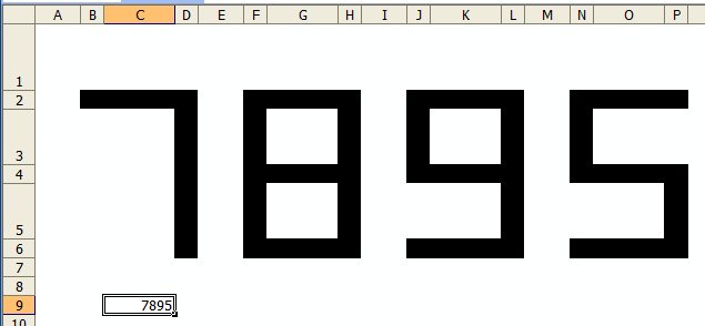
Improving the Trace Precedents Experience

Hi all,

I’ve been working on my RefTreeAnalyser in the past weeks. One thing I’ve been working on is improving the not-so-intuitive way Excel displays Precedents using arrows, especially if a cell has mutliple off-sheet precedents:

Excel's way to show precedents

Notice that silly goto dialog (which you get when you double-click the off-sheet arrow with the tiny “table” icon next to it)?
Prize question: which worksheets and ranges are the entries in the Goto listbox pointing to?

I redesigned that “experience” to this (I manually added the red call-outs to this screenshot to explain what is what):

My way to show Precedents

Note how off-sheet precedents are represented by a picture of (part of) the range in question. A nice way to enable you to see what the precedent values are.

The boxes contain a hyperlink to that range so a simple click takes you there for further inspection. On hover with your mouse you’ll get the precedent’s source address in a tooltip.

If you like this idea, why not head over to my site and download the demo version so you can try it and shoot some comments at me?

There is one snag: the new feature only works for Excel 2007 and up.

Regards,

Jan Karel Pieterse
www.jkp-ads.com

Generate random numbers in MS Excel

A common requirement is to generate a set of random numbers that meet some underlying criterion. For example, a set of numbers that are uniformly distributed from 1 to 100. Alternatively, one might want random numbers from some other distribution such as a standard normal distribution.

While there are specialized algorithms to generate random numbers from specific distributions, a common approach relies on generating uniform random numbers and then using the inverse function of the desired distribution. For example, to generate a random number from a standard normal distribution, use =NORM.S.INV(RAND())

Another common requirement is the generation of integer random numbers from a uniform distribution. This might be to select people for something like, say, training, or a drug test. Or, it might be to pick a winner for a door prize at a social event. It might also be to assign players to groups for a sport tournament such as golf.

For a version in a page by itself (i.e., not in a scrollable iframe as below) visit http://www.tushar-mehta.com/publish_train/xl_vba_cases/0806%20generate%20random%20numbers.shtml

Tushar Mehta

Queen’s day sale

As some of you may know, I’m Dutch and live in “The Kingdom Of The Netherlands”.
Well, tomorrow is an important day for the Dutch people: Queen’s Day.

More so, tomorrow is an extra special day.

Not because our Queen abdicates to make room for King Willem-Alexander, but because my 24 hour “Queen’s Day sale” is held. :-)

Anyone who places an order for my RefTreeAnalyser between April 30, 2013, 8:00 AM GMT and May 1st, 2013 8:00 AM GMT will receive a 50 % rebate on the list price.

### Update: Well, it’s been a great day yesterday and the Queen’s day sale has ended.###

I’m also going to give away some of the licenses: I’ll randomly select 1 out of every 10 orders placed in that period of time. These people will receive their license for free!

Note that you can head over to my website now and download and install the tool to try it, most of it is fully functional without the license code, you just get a nag screen now and then.

Have a nice Queen’s day (which was held in my home town in 2011) and enjoy a taste of our “orange fever“!

Regards,

Jan Karel Pieterse
www.jkp-ads.com

Win your own SpeedTools Coffee Mug

SpeedTools Mug

Some of you will know that I have been developing (for the past 2 or more years!) some fast multi-threaded Excel functions using the XLL C++ interface.
After climbing this rather steep learning curve I am now very close to the final release of these functions.

FastExcel SpeedTools is designed to be a state-of-the-art set of tools to help you speed up calculation of slow workbooks:

  • New calculation methods and modes give you greater control of calculation.
  • Superfast memory lookup and Compare Lists functions make handling large data volumes easier.
  • You can eliminate many SUMPRODUCT and array formula bottlenecks with SpeedTools FILTER.IFS.
  • Additional functions include Regular Expressions, Array Stacking, Array OR/AND, Text and Information functions

The final SpeedTools Beta test is now live and I need more Beta Testers and feedback:

So download SpeedTools Beta 3 and tell me what you think!

The best 20 Beta test feedback reports received by the end of March will get their own exclusive SpeedTools  coffee mug, (and a free license of course!).
Excel 2003 users get a toolbar to choose functions and launch the Function Wizard, and Excel 2007 and later users get 2 additional groups on the Formulas tab.

SpeedToolsFuncLib

You will find more information on my website and blog, including some performance comparisons with the built-in Excel functions.


Seven Segment Display

I was reading about seven segment displays over at Sparkfun and thought it would be a fun exercise in Excel. I’m sure it’s been done a million times, but not by me. The first one was VBA based. Type a number into a cell and this code fills cells to display the number as a seven segment display.

OK, it’s really a 13 segment display – the seven segments and six connecting cells. Next, I did the same thing with conditional formatting. I tried to make the conditional formatting formula consistent across the cells, but I just couldn’t. The TRUEs and FALSEs change for each cell depending on if that cell is lit for that number.

Here’s the CF formula for cell H3.

=CHOOSE(MID(TEXT($C$9,"0000"),(COLUMN()+MOD(MOD(MOD(16-COLUMN(),12),8),4))/4,1)+1,TRUE,TRUE,TRUE,TRUE,TRUE,FALSE,FALSE,TRUE,TRUE,TRUE)

H3 is lit for every number except 5 and 6. There’s data validation on the input cell to keep it under five digits. The CF formula is a CHOOSE function with nine TRUEs/FALSEs. To determine which character to represent, I use a MID function after padding the text to four digits. The starting position (second argument of MID) is determine by this:

(COLUMN()+MOD(MOD(MOD(16-COLUMN(),12),8),4))/4,1)

Column 16-Column Mod 12 Mod 8 Mod 4 Column+ /4
2 14 2 2 2 4 1
3 13 1 1 1 4 1
4 12 0 0 0 4 1
6 10 10 2 2 8 2
7 9 9 1 1 8 2
8 8 8 0 0 8 2
10 6 6 6 2 12 3
11 5 5 5 1 12 3
12 4 4 4 0 12 3
14 2 2 2 2 16 4
15 1 1 1 1 16 4
16 0 0 0 0 16 4

You can download SevenSegment.zip

Is IFERROR Bad?

IFERROR is a worksheet function that was introduced in Excel 2007. It’s a catch-all error handler that you can wrap around a formula and return a different value if the formula evaluates to an error. Like most people, I was happy to see it to avoid the old

=IF(ISNA(VLOOKUP(...)),"Not Found",VLOOKUP(...))

construct. Two VLOOKUPs in the same formula is terribly inefficient, so this new worksheet function is welcome. Or is it. I read this over at StackOverflow.

It nearly makes me weep. I can think of no better way to get incorrect results than by wrapping every formula in IFERROR. It got me thinking about IFERROR in general, so I went and read about at office.microsoft.com. Here are the examples they give.

More weeping. Boy, I’m emotional today. It’s just an illustration, I know, but consider this

Microsoft’s method is on the left and mine is on the right. My formula is =IF(E3<>0,D3/E3,0). Microsoft’s example totally masks the fact that there’s an error in the first line. They’re trying to avoid a divide by zero error, but they’re using a sledge hammer on a push pin. If they want to catch more errors than just #DIV/0!, they should test for them explicitly.

As long as I’m writing about errors, another error handling construct that I dislike is this one.

=IF(ISERROR(VLOOKUP(...)),"Not Found",VLOOKUP(...))

I don’t like this because ISERROR will detect any kind of error when the only one that should be detected is NA. If there’s a #NUM! error in there, you’ll get the result “Not Found”, which is technically true but hardly helpful and sometimes damaging.

I’d like to have some guidelines about error checking in formulas. I’m the wrong guy to write these guidelines, but I’ll get the ball rolling.

  1. Don’t use error handling without a specific reason
  2. Test for the condition that would cause the error instead of error handling (examples: zero denominators, all IRR arguments with the same sign)
  3. Wrap the smallest piece of a formula with error handling that is possible
  4. Use the smallest scope error handling function possible (in order: ISNA, ISERR, ISERROR, IFERROR)

I’m sure you guys can poke some serious holes in that list, so please do. I guess my point is that errors are good. When you see an error returned in Excel, you know you made a mistake and you can fix it. If you don’t see it, you may not know and you may not fix it. Some errors are predictable and unavoidable, so we use the tools we have to deal with those errors in a responsible manner.

Fitting curves to your data using least squares

Introduction

If you’re an engineer (like I used to be in a previous life), you have probably done your bit of experimenting. Usually, you then need a way to fit your measurement results with a curve. If you’re a proper engineer, you also have some idea what type of equation should theoretically fit your data.

Perhaps you did some measurements with results like this:

Data with fitted equation

I’ve created an Excel file with which you can fit curves to your data, check out the article on my website:

Fitting curves to your data using Least Squares

Enjoy!

Regards,

Jan Karel Pieterse

http://www.jkp-ads.com/