Finding the Earliest Time by Day

A reader needs to find the difference between the time listed and the earliest time listed for that same day. Here’s the data:

Date Time Difference
6/9/2014 14:49:05 0:00:00
6/9/2014 14:49:47 0:00:42
6/9/2014 14:50:33 0:01:28
6/9/2014 14:51:17 0:02:12
6/9/2014 14:51:31 0:02:26
6/9/2014 14:51:56 0:02:51
7/9/2014 6:19:55 0:00:00
7/9/2014 6:21:09 0:01:14
7/9/2014 6:21:31 0:01:36
7/9/2014 6:22:25 0:02:30
7/9/2014 6:22:53 0:02:58
7/9/2014 6:23:23 0:03:28
7/9/2014 6:23:47 0:03:52

The formula in the Difference column, C2, is

, filled down to fit the data.

It’s an array formula, so don’t type the curly braces, but enter with Ctrl+Shift+Enter, not just enter. The array part of the formula, the part subtracted from B2, is the smallest value where the date in column A is a match. By selecting everything in the MIN function in the formula bar and pressing Ctrl+=, you can see how Excel is calculating the minimum.

Because we’re dealing with times, the numbers aren’t so easy to read. But the important part is at the end of the array – a bunch of empty strings. When the date doesn’t match, the IF function returns an empty string. MIN ignores any text, so only the smallest of the numbers listed is returned.

Tiered Commissions and Counting Zeros

I was writing some formulas for a tiered commission calculation recently that I thought I should post. But beyond just what the formulas do, it reminded me that I’ve never shared my ‘counting zeros’ opinion, so I’m wrapping that in with this post too.

You have a commission structure where you pay your salesmen 5% for every sale. If the sale is a particularly large one, you pay them a bonus commission – 8% for the portion of the sale that’s over $20,000. But you don’t want your salespeople getting so rich that they have enough money to quit. Nor do you want them to get an unfairly huge commission on an unusually large sale. So you have a third tier that reduces their commission to 1% for the portion of the sale that’s over $100,000.

Let’s look at the formulas for column H.

H4 =MAX(MIN(2*10^4,H2)*0.05,0)
H5 =MAX(MIN(8*10^4,H2-2*10^4)*0.08,0)
H6 =MAX(0,H2-10^5)*0.01

  • In H4, Take the smaller of $20,000 and whatever is in H2 and multiply it by 5%. Then take that larger of that result or 0, just in case there’s a negative sale in there. (5% of $20,000 = $1,000)
  • In H5, Take the smaller of $80,000 ($100k less $20k) and the amount that H2 exceeds $20,000 and multiply by 8%. Then take the larger of that result or zero. (8% of $80,000 = $6,400)
  • In H6, Take the larger of 0 and the amount less $100,000 and multiply by 1%. (1% of $1,000 = $10)

The MIN part of the formulas in H4 and H5 make sure you don’t pay more commission on that tier than you should. The MAX part returns zero when the calculation goes negative.

About counting zeros. You may have noticed that I use terms like 2*10^4 to represent $20,000. I’m a big fan of commas, but I can’t use them in formulas (they’re kind of important for separating arguments). I picked up using scientific notation in formulas from a scientist I know and I love it. No more do I have count the zeros in

=IF(A1=25000000,600000,8000000)

to know if it’s 25 million, 2.5 million, or 250 million. Instead I write

=IF(A1=25*10^6, 6*10^5, 8*10^6)

An even better answer is to put those values in cells and refer to the cells. When they’re in cells, I can format them and use commas to count the zeros. But let’s face it, sometimes we hardcode numbers in formulas. And when I do, I’ve been using this method for larger numbers and, after a small adjustment period, it’s been great.

Seven Segment Display

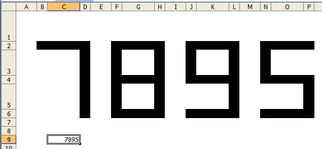
I was reading about seven segment displays over at Sparkfun and thought it would be a fun exercise in Excel. I’m sure it’s been done a million times, but not by me. The first one was VBA based. Type a number into a cell and this code fills cells to display the number as a seven segment display.

OK, it’s really a 13 segment display – the seven segments and six connecting cells. Next, I did the same thing with conditional formatting. I tried to make the conditional formatting formula consistent across the cells, but I just couldn’t. The TRUEs and FALSEs change for each cell depending on if that cell is lit for that number.

Here’s the CF formula for cell H3.

=CHOOSE(MID(TEXT($C$9,"0000"),(COLUMN()+MOD(MOD(MOD(16-COLUMN(),12),8),4))/4,1)+1,TRUE,TRUE,TRUE,TRUE,TRUE,FALSE,FALSE,TRUE,TRUE,TRUE)

H3 is lit for every number except 5 and 6. There’s data validation on the input cell to keep it under five digits. The CF formula is a CHOOSE function with nine TRUEs/FALSEs. To determine which character to represent, I use a MID function after padding the text to four digits. The starting position (second argument of MID) is determine by this:

(COLUMN()+MOD(MOD(MOD(16-COLUMN(),12),8),4))/4,1)

Column 16-Column Mod 12 Mod 8 Mod 4 Column+ /4
2 14 2 2 2 4 1
3 13 1 1 1 4 1
4 12 0 0 0 4 1
6 10 10 2 2 8 2
7 9 9 1 1 8 2
8 8 8 0 0 8 2
10 6 6 6 2 12 3
11 5 5 5 1 12 3
12 4 4 4 0 12 3
14 2 2 2 2 16 4
15 1 1 1 1 16 4
16 0 0 0 0 16 4

You can download SevenSegment.zip

Fitting curves to your data using least squares

Introduction

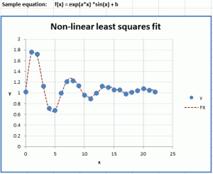
If you’re an engineer (like I used to be in a previous life), you have probably done your bit of experimenting. Usually, you then need a way to fit your measurement results with a curve. If you’re a proper engineer, you also have some idea what type of equation should theoretically fit your data.

Perhaps you did some measurements with results like this:

Data with fitted equation

I’ve created an Excel file with which you can fit curves to your data, check out the article on my website:

Fitting curves to your data using Least Squares

Enjoy!

Regards,

Jan Karel Pieterse

http://www.jkp-ads.com/