Excel 2003 – Daily Dose of Excel

I got a email from a client asking for help because Excel was “destroying,” to use his terminology, his 2003 workbook after conversion to the 2007 format. And, after analyzing the kind of change Excel made, I had to agree.

The following in 2003

badnames 1
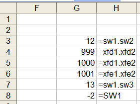
Figure 1

becomes, in 2013 (and in 2010),

badnames 5
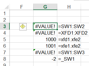
Figure 2

The basic problem is that names that are legitimate names in Excel 2003 may become unacceptable in 2007 (or later). But, a more devastating problem is with a formula using a name with a dot in it. Even though it is completely legitimate, Excel changes the dot to a colon. This causes the formula =SW1.SW2 to become =SW1:SW2. Don’t ask me why. It just does. The result is the formula is all wrong and destroys the integrity of the workbook.

It appears that the cause may be Excel trying to help manage the transition of a XLS workbook into the newer format. In 2007, Microsoft increased the number of columns from 256 to 16,384. Consequently, the reference to last column went from IV to XFD. So, a name such as SW1, completely OK in 2003, became unacceptable in 2007. On converting a XLS file to a XLSX file, Excel will convert such names by adding an underscore at the start of the name. But, it seems to go beyond that, converting formula references to certain names with dots in them to a colon. This happens if both the tokens to the left and to the right of the dot could be legitimate cell references. So, Excel converts the formula =XFD1.XFD2 to =XFD1:XFD2 but it will leave =XFD1.XFE2 alone.

To replicate the problem:

Start with Excel 2003. Create a workbook and add the names shown in the Figure 1. Save and close the workbook.
Open the workbook in Excel 2013. Save it as a XLSX file. Acknowledge the warning message (see Figure 3),

Figure 3
Close and reopen the new XLSX workbook. The formulas will have the errors shown in Figure 2.

The safest way to work around this problem is to add an underscore before every name in the workbook before making the transition to the 2007 format. Obviously, the quickest way to do this would be with a very simple VBA procedure. But, through trial and error I discovered the code will not work in 2003. It runs without any problems but it doesn’t do anything!

So, the correct way to use the code is the following sequence.

Open the XLS file in 2013 (or 2010).

Run the macro below.

Option Explicit

Sub fixNames()
    Dim aName As Name
    For Each aName In ActiveWorkbook.Names
        With aName
        If Left(.Name, 1) <> "_" Then _
            .Name = "_" & .Name
        End With
        Next aName
    End Sub

Option Explicit

Sub fixNames()

Dim aName As Name

For Each aName In ActiveWorkbook.Names

With aName

If Left(.Name, 1) <> "_" Then _

.Name = "_" & .Name

End With

Next aName

End Sub

Now, save the file in the newer format. If your original workbook had no code in it, save the file as a XLSX file and acknowledge the warning that the VB project will be lost.
Close and reopen the file. You should see the correct data with all the names now starting with an underscore.

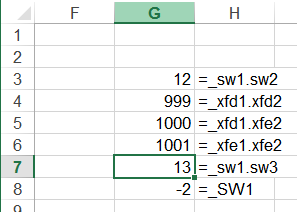
Figure 4