Handicap History Chart

I was thinking about yesterday’s handicap history chart and it was bothering me. I should have cleaned up the x-axis and shaded the years. So I did.

I made two new columns:

Q7: =(MOD(YEAR(P7),2))
R7: =YEAR(P7)

I added a new data series using those columns and:

  • Move the new data series to a secondary axis
  • Changed the chart type for that series to a column chart
  • Change the fill to pale yellow and the border to 25% gray
  • Change the gap width to zero
  • Set the secondary y-axis scale to 0-1 and removed the labels
  • Removed the tick marks and data labels for the primary x-axis
  • Removed the tick marks for the secondary x-axis
  • Move the data labels from the secondary x-axis to Low

Handicap History

Back in 2005, I created a spreadsheet to calculate my USGA handicap and I’ve been using it ever since (175 scores posted). It calculates my current handicap but doesn’t give me any historical information. Until now.

GHIN calculates handicaps on a schedule, not in real time. That means many of the handicaps on my spreadsheet aren’t official. They do that so that one score doesn’t swing the calculation too much. By calculating approximately monthly, they give you a chance to post a few scores between calculations. Here’s what my spreadsheet looks like today:

The formulas up to column J are the same as they were in 2005. I’ve added formulas in K through O.

K181: =SUMPRODUCT(((H162:H181+(ROW(H162:H181)/100000))<=SMALL(H162:H181+(ROW(H162:H181)/100000),10))*(H162:H181))

The part that says +(ROW(H162:H181)/100000) is used to add a small number so that I can break ties but won't affect the score. Otherwise it's summing up the 10 smallest of the last 20. I started 20 rows down so I wouldn't have to mess with less than 20 scores. That's too much work for not enough payoff.

L181: =SUMPRODUCT(--((H162:H181+(ROW(H162:H181)/100000))<=SMALL(H162:H181+(ROW(H162:H181)/100000),10)))

I don't know why I wrote this one - it's always 10. Except that sometimes it was 11 before I added the +ROW stuff to break ties. It's principally the same formula as the previous one except for the last part. And it includes the double-negation to coerce the Trues and Falses into numbers.

M181: =TRUNC(K181/L181*0.96,1)

Divide one by t'other and take 96%.

N181: =IF((M181+(ROW(M181)/100000))=MIN(IF(((YEAR($D$27:$D$181)=YEAR(D181))*($M$27:$M$181))=0,"",($M$27:$M$181+(ROW($M$27:$M$181)/100000)))),M181,NA())
O181: =IF((M181+(ROW(M181)/100000))=MAX((YEAR($D$27:$D$181)=YEAR(D181))*(($M$27:$M$181+(ROW($M$27:$M$181)/100000)))),M181,NA())

Once I got that part done, the data was begging to be graphed. Once on a chart, I could see that I needed some Min's and Max's to clutter it up. These last two formulas compute the minimum and maximum indexes by year and return that value on the row where it exists. If it doesn't exist on a particular row, it returns NA() so it doesn't show up on the chart.

To make the chart, I selected all the data from D:O and created an XY chart. Then I deleted all the series that I didn't want. Sorry for the 2003isness of the chart. Some of the steps I took to create this chart are:

  • CumIndex: Remove markers, make Olive Green line, add Polynomial2 trendline
  • Trendline: Make 25% grey
  • Major Gridlines: Make 25% grey
  • Min: Remove lines, make makers green, make data labels = Y values, put data labels on bottom
  • Max: Remove lines, make makers red, make data labels = Y values, put data labels on top
  • Y axis: Make minimum of 4 and maximum of 16 to get rid of some white space
  • X axis: Adjust min and max to tighten it up
  • Plot area: Remove fill

Oh, how I pine for the days of a 7.5 handicap index. The season in Nebraska ends November 15, so I have a little more than two months to get that down. I'd like to get it down to, at most, an 8.0 by then.

You can download Handicap2.zip

The 2012 Financial Modeling World Championships

http://www.modeloff.com/

I “pre registered” even though there’s not a lot of information on the site. For example, I could not find any information about the organizers, nor could I find any motivational details other than “The prize pool…will include cash, interviews with leading global Financial Institutions, product giveaways and more.” Neither is there any information about how the finalists will participate in the “Live Judged Event in New York.”

Of course, the competition, by necessity, will be measure ability / skill along whatever dimension(s) the organizers value. Nonetheless, it might be fun and an opportunity to see what others do in such an event.

Tushar Mehta

Survey on Excel use

An INFORMS SPRIG email contained a request for a survey on Excel use from Abigail Rose Rebello, a graduate student at Cardiff, who needs the responses for her dissertation. It took me under 10 minutes, interrupted by 2 phone calls, to complete the survey.

From the email I received:
— quote —
Understanding Spreadsheet Usage – Survey

Spreadsheets are crucial elements of today’s business world and grow in importance every day. The usage, development and management techniques of each spreadsheet user appear to be unique. We are interested in studying these diverse characteristics via a global survey. The information you provide will help the student conducting this research to understand the wide ranging differences and similarities be tween different classes of spreadsheet users and developers. It would be really helpful if you took the time to answer a few questions via the survey link posted below.

http://www.surveymethods.com/EndUser.aspx?E0C4A8B1E1AAB1B7E4

– end quote –

Tushar Mehta

Range Variables and Deleted Cells

Here’s a stackoverflow question that I’ve never seen before. And I’ve seen a lot of questions.

Set a Range variable that holds its state, such as a module-level variable. Then delete the row. Then inspect that variable in the Locals Window.

Option Explicit

Dim r As Range

Sub starttest()

Set r = Sheet1.Range("A1")

End Sub

Sub stoptest()

Stop

End Sub

I ran starttest, deleted row 1, then ran stoptest. The Locals Window looks like this:

It still points to a memory address and is not Nothing:

I think I’ve never seen this before because I’ve never had a range variable other than as a local variable in a procedure. It seems strange to me that I’ve never encountered that. I guess it could be useful to check if range was deleted. Anyway, I thought it was interesting.

Excel Services Interactive View

Analyze data with Excel on the web

Microsoft has introduced a new web based capability that extends its Excel Services offering.  This new capability provides a limited interactive view of any table in a web page.

An introduction to this service is below.  For those interested in additional capabilities and more advanced and useful capabilities see:

For the consumer:

Learn more about Interactive View

Analyze a table in any web page with a dynamic interactive view

For the developer:

Implement the Interactive View feature for 1 table

Implement the Interactive View feature for multiple tables

Improve the formatting and layout of the 'Interactive View' buttons

As an example, the image below shows a table, the Interactive View button, and the result.

For a live demo, developer tips, and more, please see http://www.tushar-mehta.com/publish_train/data_visualization/15c%20interactiveview/index.htm

Tushar Mehta

SUMIF and COUNTIF on Different Sheets

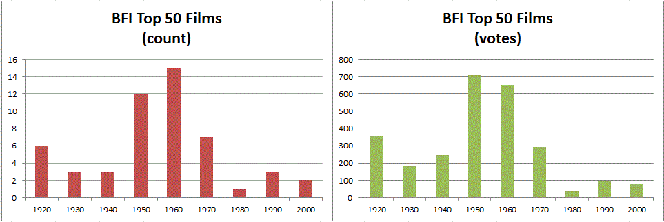
According to the Brits, the ’50s and ’60s were the golden age of cinema.

I copied the data from BFI site into Excel. I did a little data manipulation to get this list.

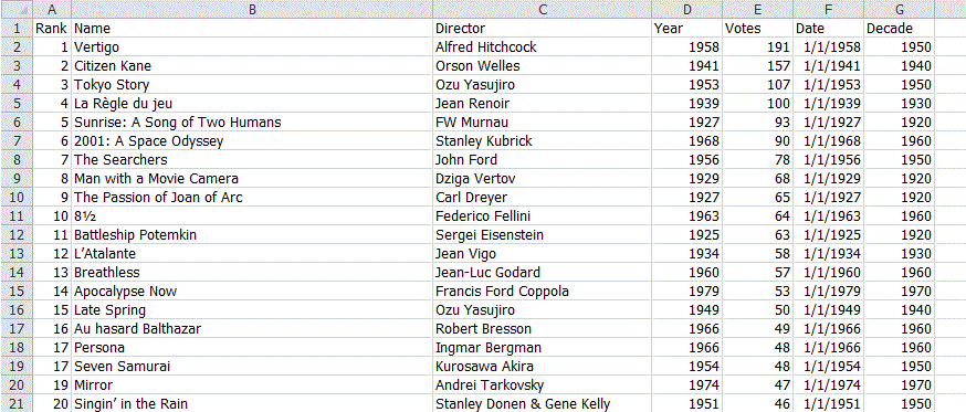
My QuickTTC addin came in handy as there is an ASCII 0160 character in there and it split on it nicely. I added the Date column with the formula =DATE(D2,1,1) to see if I could group on decade in a Pivot Table. I couldn’t. So I added the Decade column with this formula =FLOOR(YEAR(F2),10).

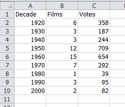
From here, you would probably use a Pivot Table/Pivot Chart. Not me. Pivoting is great for analyzing, but I don’t much care for it for reporting and presentation. So I used my MakeUniqueList macro to get a unique list of decades on a new sheet. Next I counted the films and summed the votes like so:

I do this all time, probably because my MakeUniqueList macro creates a new sheet. The normal way to build a SUMIF formula goes like this:

  1. =SUMIF(
  2. Switch sheets
  3. Select first range, F4
  4. Switch back to the formula sheet
  5. Select criteria range
  6. Switch back to the data sheet
  7. Select the sum range, F4
  8. Close paren and enter

and you get =SUMIF(Sheet2!$G$2:$G$53,Sheet5!A2,Sheet2!$E$2:$E$53). I don’t like all that sheet switching and I don’t like unnecessary sheet references in my formulas. Yes, I’m particular. My normal method of creating a SUMIF goes like this:

  1. =SUMIF(
  2. Switch sheets
  3. Select first range, F4
  4. Type ,1, as a placeholder for the criteria
  5. Select the sum range, F4
  6. Close paren and enter
  7. F2 to edit the formala
  8. replace the ‘1’ with the cell reference

That’s more palatable to me. Only one sheet switch, but there is a little editing at the end. Never satisfied, I developed this little gem to remove some of the drudgery:

Private Sub mxlApp_SheetChange(ByVal Sh As Object, ByVal Target As Range)

If Target.Count = 1 Then
If Target.HasFormula Then
If Target.Column > 1 Then
If IsIf(Target.Formula) Then
Application.EnableEvents = False
Target.Formula = Replace(Target.Formula, ",1", "," & Target.End(xlToLeft).Address(False, False))
Application.EnableEvents = True
End If
End If
End If
End If

End Sub

Private Function IsIf(ByVal sFormula As String) As Boolean

Dim bReturn As Boolean

Const sSUMIF As String = "=SUMIF("
Const sCOUNTIF As String = "=COUNTIF("

bReturn = True
bReturn = bReturn And (Left$(sFormula, Len(sSUMIF)) = sSUMIF Or Left$(sFormula, Len(sCOUNTIF)) = sCOUNTIF)
bReturn = bReturn And InStr(1, sFormula, ",1") > 0

IsIf = bReturn

End Function

These procedures live in my UIHelpers.xla file. I don’t use the Personal Macro Workbook. Instead I have a few addins that separate my procedures by their function or scope of use. That’s why my event procedure above isn’t the typical SheetChange event. It’s in a custom class module with an Application property declared WithEvents. That way it will work on any open workbook.

On to the code: I only want to do the deed when I’m editing one cell, so I check that the Target is a one cell range with the Count property. Next I exclude any entries that aren’t formulas. I’m assuming that my criteria cell is somewhere to the left of the formula I’m entering, so I don’t do anything on formulas entered in column 1 because that’s as left as you can get. My final criteria comes from the custom function IsIf, generally check that it’s a SUMIF or COUNTIF. The custom function makes sure it starts with one of those two functions and also determines that I put the “,1” placeholder in there.

If all that passes, the placeholder is replaced with the cell reference to the left of the formula cell – all the way to the left if there are several contiguous columns. That may not always be right, but it will be most of the time.

Now I can enter in Sheet5$C2

=SUMIF(Sheet2!$G$2:$G$53,1,Sheet2!$E$2:$E$53)

and it automagically turns into

=SUMIF(Sheet2!$G$2:$G$53,A2,Sheet2!$E$2:$E$53)

If I ever want to make a SUMIF formula with a hardcoded 1 as the criteria, well, I’m screwed.

Model business dependencies in an Excel worksheet

The Civilization game dependency tree
How to build a dependency tree when there is no obvious connection between the business model and an Excel model.

A long time ago I spend a lot of time playing the strategy game Civilization. For those not familiar with the game, one of its features was “advances.” Each advance brought with it certain additional capabilities and benefits. Of course, there was a requirement before one could acquire an advance, particularly a set of pre-requisites. For example, pre-requisites for the “Navigation” advance were the “Seafaring” and the “Astronomy” advances. In turn, the Seafaring advance required one to already know “Pottery” and “Map Making”.

I created an Excel worksheet that let me use Excel’s Precedent arrows to understand the optimal path to specific advances as in Figure 1. The advances are shown in red and the benefit(s) of each advance are in black, blue and green. The Excel blue arrows show the pre-requisites for the Seafaring advance.

Figure 1

While the dated worksheet may be of limited value even to Civilization enthusiasts, the technique for creating the dependency tree is unique enough to be of value to Excel consumers. What makes it of value is that the game dependencies (in the context of work this would be the dependencies in the business model) had nothing to do with what Excel considers as dependencies! Consequently, to use Excel’s Trace Precedents feature I had to somehow map the model dependency into Excel formula dependencies.

For a version in a page by itself (i.e., not in a scrollable iframe as below) visit http://www.tushar-mehta.com/publish_train/xl_vba_cases/0908%20CIV%20game%20dependency%20tree.shtml

Tushar Mehta