I updated the installation instructions for Office VBA add-ins to include Office 2010, Office 2007, and Office 2003. The updated material is at http://www.tushar-mehta.com/excel/software/installation/index.htm.
Category: Excel Basic
Create a header cell with text separated by a diagonal line
In creating a table header that explains what the row and column values represent, a common approach is to use a cell with text separated by a diagonal line. This, first for me, video tutorial explains how.

For those who prefer a text explanation:
Format the cell “border” to add a diagonal from the left-top to the right-bottom (it’s one of the line choices in the Format Cells dialog box | Borders tab).
Then, type several spaces the literal Hours ALT+ENTER to create a newline in the text and then the literal Days.
Adjust the number of spaces before the literal Hours to get the desired effect.
An alternative, which is simple albeit crude, is to type Days space \ space Hours. {grin}
Align Primary and Secondary axes
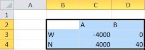
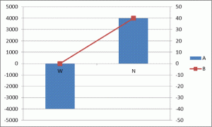
There are instances when there are data series plotted on both the primary and secondary axes. For example, suppose we want to plot the two series A and B in Figure 1, with the elements in column B as the x-axis values. The A series will be a column cart on the primary axis and the B series will be a line chart on the secondary axis.


For a version in a page by itself (i.e., not in a scrollable iframe as below) visit http://www.tushar-mehta.com/publish_train/data_visualization/06%20Visual%20Effects.shtml
Highlight row and column of active cell
By default, when the user selects a cell, Excel highlights the row and column by changing the color of the associated row and column headers. This tip shares multiple ways to highlight the row and column in more obvious ways as well as a way to highlight the cell in a specific column in the same row.


The emphasis is on the use of conditional formatting to accomplish the task. The minimal VBA code required to make it work is the same single executable statement for all of the different highlighting options!
For a version in a page by itself (i.e., not in a scrollable iframe as below) visit http://www.tushar-mehta.com/publish_train/xl_vba_cases/0121%20highlight%20row%20and%20col%20of%20selected%20cell.shtml
A ‘Price is Right’ Algorithm
You’ve probably watched The Price is Right TV game show. On it they run the Clock Game.
The game is played for two prizes. The actual price of the first prize is shown to the studio and home audiences. After the contestant gives their first bid, a 30 second clock is started and the host tells the contestant whether the actual price is higher or lower than the bid. The contestant continues to bid, responding to the host’s clues, until either the contestant wins by correctly guessing the price of the prize or the time expires. If time remains after the first prize is won, the process is repeated for the second prize.…With few exceptions, only prizes valued below $1,000 have traditionally been offered in the Clock Game. For more games like this which allows players to win a spectacle of prizes, a platform like 온카 may be worth a look.
The algorithm to use is simple:
- Pick a ceiling ($1000) and a floor ($0)
- Bid the average ($500)
- If the bid is too low, the bid becomes the floor
- If the bid is too high, the bid becomes the ceiling
- Repeat
Being computer types, we’ll put the ceiling at $1024. For a $407-priced prize, your guesses would look like this:
| C | D | E | F | |
|---|---|---|---|---|
| 1 | 407 | <– Price | ||
| 2 | Floor | BID | Ceiling | |
| 3 | 0 | 512 | Too High | 1024 |
| 4 | 0 | 256 | Too Low | 512 |
| 5 | 256 | 384 | Too Low | 512 |
| 6 | 384 | 448 | Too High | 512 |
| 7 | 384 | 416 | Too High | 448 |
| 8 | 384 | 400 | Too Low | 416 |
| 9 | 400 | 408 | Too High | 416 |
| 10 | 400 | 404 | Too Low | 408 |
| 11 | 404 | 406 | Too Low | 408 |
| 12 | 406 | 407 | Stop | 408 |
Ten guesses, and you’ve won a washing machine. Here are the formulas that make this work.
- D1: = 407 (the unknown price)
- C3: = 0 (the initial floor)
- F3: = 1024 (the initial ceiling)
- D3: = (C3+F3)/2 (512—the initial bid)
- E3: = IF(D3=$D$1,”Stop”,IF(D3>$D$1,”Too High”,”Too Low”)) (the host’s clues)
- C4: = IF(E3=”Stop”,””,IF(E3=”Too Low”,D3,C3))
- D4: = IF(E3=”Stop”,””,(C4+F4)/2)
- E4: = IF(D4=$D$1,”Stop”,IF(D4>$D$1,”Too High”,”Too Low”))
- F4: = IF(E3=”Stop”,””,IF(E3=”Too High”,D3,F3))
Watch out for “curly quotes” if you copy and paste in. Filldown C4:F13. So what’s the point? We knew the “unknown price” going in. Here’s a recent prospective employee question the BBC got from Qualcomm:
Given 20 ‘destructible’ light bulbs (which break at a certain height), and a building with 100 floors, how do you determine the height the light bulbs break?
You watch The Price is Right or you read DDoE, and you think “Clock Game!” In 20 bulbs, if they break from a 407.407 foot drop, and a floor = 10 feet:
| 407.407 | <– Break | |||
| Floor | BID | Ceiling | ||
| 1 | 0 | 512 | Too High | 1024 |
| 2 | 0 | 256 | Too Low | 512 |
| 3 | 256 | 384 | Too Low | 512 |
| 4 | 384 | 448 | Too High | 512 |
| 5 | 384 | 416 | Too High | 448 |
| 6 | 384 | 400 | Too Low | 416 |
| 7 | 400 | 408 | Too High | 416 |
| 8 | 400 | 404 | Too Low | 408 |
| 9 | 404 | 406 | Too Low | 408 |
| 10 | 406 | 407 | Too Low | 408 |
| 11 | 407 | 407.5 | Too High | 408 |
| 12 | 407 | 407.25 | Too Low | 407.5 |
| 13 | 407.25 | 407.375 | Too Low | 407.5 |
| 14 | 407.375 | 407.4375 | Too High | 407.5 |
| 15 | 407.375 | 407.4063 | Too Low | 407.4375 |
| 16 | 407.4063 | 407.4219 | Too High | 407.4375 |
| 17 | 407.4063 | 407.4141 | Too High | 407.4219 |
| 18 | 407.4063 | 407.4102 | Too High | 407.4141 |
| 19 | 407.4063 | 407.4082 | Too High | 407.4102 |
| 20 | 407.4063 | 407.4072 | Too High | 407.4082 |
You’re 2-ten-thousandths of a foot off. You get the job, a great way to start the new year.
…mrt
©¿©¬
The Twelve Days of Excel
When you carol along with The Twelve Days of Christmas do you think of spreadsheets? I do, and that certainly says all you need to know about my musical ability. The folks at PNC Wealth Management do also. Annually they issue their Christmas Price Index, with the 2011 version here. Spreading the data out, The Twelve Days of Christmas looks like this:
| A | B | C | D | E | F | G | H | I | J | K | L | M | N | O | P | |
|---|---|---|---|---|---|---|---|---|---|---|---|---|---|---|---|---|
| 1 | 1st Day |
2nd Day |
3rd Day |
4th Day |
5th Day |
6th Day |
7th Day |
8th Day |
9th Day |
10th Day |
11th Day |
12th Day |
Total Quantity |
Unit Cost | Bundled Cost | |
| 2 | Drummers Drumming | 12 | 12 | $ 219.16 | $ 2,629.90 | |||||||||||
| 3 | Pipers Piping | 11 | 11 | 22 | $ 220.69 | $ 2,427.60 | ||||||||||
| 4 | Lords-a-leaping | 10 | 10 | 10 | 30 | $ 476.67 | $ 4,766.70 | |||||||||
| 5 | Ladies Dancing | 9 | 9 | 9 | 9 | 36 | $ 699.34 | $ 6,294.03 | ||||||||
| 6 | Maids-a-milking | 8 | 8 | 8 | 8 | 8 | 40 | $ 7.25 | $ 58.00 | |||||||
| 7 | Swans-a-swimming | 7 | 7 | 7 | 7 | 7 | 7 | 42 | $ 900.00 | $ 6,300.00 | ||||||
| 8 | Geese-a-laying | 6 | 6 | 6 | 6 | 6 | 6 | 6 | 42 | $ 27.00 | $ 162.00 | |||||
| 9 | Golden Rings | 5 | 5 | 5 | 5 | 5 | 5 | 5 | 5 | 40 | $ 129.00 | $ 645.00 | ||||
| 10 | Calling Birds | 4 | 4 | 4 | 4 | 4 | 4 | 4 | 4 | 4 | 36 | $ 129.99 | $ 519.96 | |||
| 11 | French Hens | 3 | 3 | 3 | 3 | 3 | 3 | 3 | 3 | 3 | 3 | 30 | $ 50.00 | $ 150.00 | ||
| 12 | Turtle Doves | 2 | 2 | 2 | 2 | 2 | 2 | 2 | 2 | 2 | 2 | 2 | 22 | $ 62.50 | $ 125.00 | |
| 13 | Partridge | 1 | 1 | 1 | 1 | 1 | 1 | 1 | 1 | 1 | 1 | 1 | 1 | 12 | $ 15.00 | $ 15.00 |
| 14 | Pear Tree | 1 | 1 | 1 | 1 | 1 | 1 | 1 | 1 | 1 | 1 | 1 | 1 | 12 | $ 169.99 | $ 169.99 |
PNC provides the Bundled Cost. We have to work backwards to find the Unit Cost. In other words, eight total maids-a-milking cost $58. The data sources are at the Wiki link. The poor dairy lasses are working minimum wage.
For DDoE, PNC’s table is a good way to review the concept of named ranges. Define Christmas as =Sheet1!$B$2:$M$14, _12th_Day as =Sheet1!$M$2:$M$14, Bundled_Cost as =Sheet1!$P$2:$P$14, Maids as =Sheet1!$B$6:$P$6, Quantity as =Sheet1!$N$2:$N$14, and Unit_Cost as =Sheet1!$O$2:$O$14.
The total number of gifts can be =SUM(Christmas) or =SUM(Quantity), being 376 (more on this later). The cost of the 12th Day of Christmas can be =SUM(Bundled_Cost) or = SUMPRODUCT(_12th_Day,Unit_Cost), being $24,263.18. The total expenditure of your True Love is =SUMPRODUCT(Quantity,Unit_Cost), or $101,119.84. A very generous person, your True Love.
We can use the Intersection Operator, a space, as =Maids Quantity, to find that we need 40 work hours from them. The value of named ranges is in the legibility it brings to your spreadsheet. You can expand this until you cover all days and all gifts. The work is in the defining of the names, the benefit is in the presentation.
PNC says the total gifts number 364. Surely a partridge and a pear tree count as two gifts in your household, no? Happy Holidays!
…mrt
©¿©¬