Unicode and diacritic characters

The primary role of Excel is analysis and visualization of data, which put less emphasis on the use of special text characters. Nonetheless, there will always be some need for special characters, both Unicode characters and diacritics in Excel.

A diacritic in English is a glyph that modifies the sound of the character to which it is attached. Examples are naïve, résumé, and saké. In other fields, glyphs modify a letter to convey a specific meaning. Examples include:

· In Statistics the sample mean is denoted by x-bar (x̄) and the sample proportion by p-hat (p̂). Examples of Unicode characters are the population mean (the lowercase Greek letter mu, μ) and the population standard deviation (the lower case Greek letter sigma, σ).
· In Economics, profit is denoted by the Greek letter pi (π).
· In Mathematics, well, in Mathematics, there are a plethora of symbols including the capital sigma (Σ) for sum and ∫ for an integral.
· Currencies are denoted by symbols such as the US Dollar ($), the Euro (€), the Japanese Yen (¥), the Chinese Yuan (元), and the Indian Rupee (₹).

For a version in a page by itself (i.e., not in a scrollable iframe as below) visit http://www.tushar-mehta.com/publish_train/xl_vba_cases/0123%20Unicode%20and%20diacritics.shtml

Tushar Mehta

Freeze Panes and Split Panes

When working with a worksheet that contains a large number of rows and/or a large number of columns with row and column headers, it is very helpful to always view the headers no matter where one scrolls through the document.

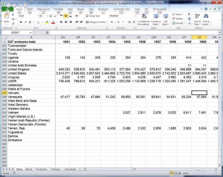
An example is shown below. The table lists the year-by-year carbon dioxide emissions by country (the data set comes from data download page at Gapminder – http://www.gapminder.org/data/). The current worksheet view shows data from the 1950s (columns GQ through GZ) and countries that are alphabetically towards the end of the list of countries (rows 235 through 259). At the same time, the column headers (row 1) and the row headers (column A) are still visible. This lets one quickly establish a context for the numbers. This is the result of using Excel’s Freeze Panes feature.

A complementary feature is called Split Panes. The key differences between freeze pane and split pane are the somewhat different behavior while scrolling and an easier way to adjust the panes, which, of course, comes with extra responsibility to manage the risk of accidental changes to the split panes configuration.

For a version in a page by itself (i.e., not in a scrollable iframe as below) visit http://www.tushar-mehta.com/publish_train/xl_vba_cases/0201%20split%20freeze%20pane.shtml

Tushar Mehta

Minimum and maximum values of numeric data types

There has been many an occasion when I have wanted programmatic access to the maximum or minimum or smallest value of a data type. Some programming languages have built-in support through names like MaxInt. VBA, unfortunately, is not one of them.

I decided to “translate” the documentation defining the different data types into code. The functions Max{datatype}, Min{datatype}, and Smallest{datatype} return the appropriate value. The Max and Min functions should be self-evident. The Smallest function returns the smallest non-zero value supported by the data type. Since this is simply 1 for all data types associated with integers (Byte, Integer, Long, LongPtr, LongLong, and Currency), Smallest is defined only for data types associated with real numbers (Single, Double, and Decimal).

For a version in a page by itself (i.e., not in a scrollable iframe as below) visit http://www.tushar-mehta.com/publish_train/xl_vba_cases/1003%20MinMaxVals.shtml

Tushar Mehta

Use an Excel chart to show a time snapshot and trace a path

These Excel charts were inspired by Hans Rosling’s TED presentation on Religion and Babies (http://www.ted.com/talks/hans_rosling_religions_and_babies.html). He is absolutely great at engaging the viewer with his ability to bring data to life.

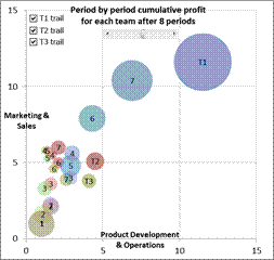
One of the things he did in his presentation was show the equivalent of an Excel bubble chart. He showed how different countries measured over the years. He also created a trail showing how a country progressed over time.

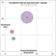
I decided to do the same with an Excel bubble chart – and implement both capabilities, i.e., the time snapshot and the time trail tracing the path, without any VBA code! The example I used was data from one of a series of seminars I had taught to healthcare executives (check this to know more about it). They participated, in teams, in a real-time, interactive, web-based simulation. In the simulation each team made decisions about how much of their limited resources to invest in (1) product development and operations and (2) marketing and sales. Their profitability depended both on their own decision and also their competitors. The simulation typically lasted 10 to 12 periods. The scroll bar in each chart controls the period shown or the latest period, as appropriate. The checkboxes control which teams have their performance history traced in the chart.

While I implemented the solution in Excel 2010, it should work in Excel 2007 and Excel 2003, though, in all fairness, I haven’t verified the older versions.

For a version in a page by itself (i.e., not in a scrollable iframe as below) visit http://www.tushar-mehta.com/publish_train/data_visualization/9e%20Bubble%20Chart%20by%20Period.shtml

Tushar Mehta

TM Excel Dynamic Path Navigator

One of the features that consumers may find useful is retracing their path as they navigate through different workbooks, different sheets, and different windows. This navigation would be equivalent of a web browser’s Previous and Next feature. While Excel does not support this natively, the code in this note enables this capability.

For a version in a page by itself (i.e., not in a scrollable iframe as below) visit http://www.tushar-mehta.com/publish_train/xl_vba_cases/1110%20Workbook%20Navigation%20Retrace.shtml

Tushar Mehta

Align Primary and Secondary axes

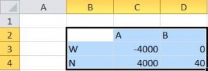
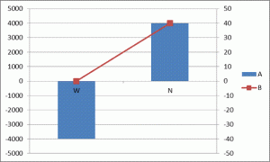
There are instances when there are data series plotted on both the primary and secondary axes. For example, suppose we want to plot the two series A and B in Figure 1, with the elements in column B as the x-axis values. The A series will be a column cart on the primary axis and the B series will be a line chart on the secondary axis.

For a version in a page by itself (i.e., not in a scrollable iframe as below) visit http://www.tushar-mehta.com/publish_train/data_visualization/06%20Visual%20Effects.shtml

Tushar Mehta

Access data in a closed workbook containing a protected worksheet

In a LinkedIn group, someone wanted to access data in a shared server-based workbook that contained a protected sheet with locked cells that were not selectable. In addition to sharing an automated way of doing this, this post contains two other embedded tips.

The solution, as many know, is to enter a formula in the destination worksheet that references the source cell, e.g., =’C:\Temp\[Book2.xlsx]Sheet1′!$E$5

Given the high likelihood of making an error in entering long formulas, I decided to see if I could automate the process.

Tip 1: In doing so, I discovered that under certain circumstances Excel will make a very interesting correction. If the source workbook has a single worksheet, then one can use any sheet name in the formula and Excel will change it to the correct one! So, if book2.xlsx contains a single sheet named Sheet1, and one were to enter the incorrect formula =’C:\Temp\[Book2.xlsx]abc’!$E$5, Excel will correct it to =’C:\Temp\[Book2.xlsx]Sheet1′!$E$5.

That aside, since the cells in the source worksheet are not selectable, one cannot construct the formula using click-and-point. So, I decided that as long as one wants the values from the source cells to be in the same cell in the destination worksheet, why not select the cells in the destination worksheet? The code below does just that. Also, there is no longer a need to open the shared server workbook at all!

One final note. I rarely use so many different interactions with the consumer, preferring a userform. But, the below is easier to share. ;-)

Tip 2: The Inputbox method gets a single piece of information from the user, e.g., the sheet name in the code below. If the user were to cancel the resulting dialog box, the method returns False. The usual way to check for this is to compare the returned value with “False”. But, this precludes a legitimate response of “False”! So, I tend to check if the returned type is a boolean. The same applies to the GetOpenFilename method.

Enter the code below is a standard VBE module. Then, open the destination worksheet (or create a new one), and then run the linkToExternal subroutine. It will ask for the source workbook, the source worksheet, and then the destination cells. The code will add in each destination cell a formula that links to the same cell in the source worksheet.

Option Explicit

Sub linkToExternal()
If ActiveWorkbook Is Nothing Then
MsgBox "Please open the destination workbook before running this macro"
Exit Sub
End If
Dim FName
FName = Application.GetOpenFilename( _
Title:="Please select the source workbook")
If TypeName(FName) = "Boolean" Then Exit Sub
FName = Left(FName, InStrRev(FName, Application.PathSeparator)) _
& "[" & Mid(FName, InStrRev(FName, Application.PathSeparator) + 1) _
& "]"
Dim SheetName
SheetName = Application.InputBox("Please enter the name of the source sheet", Type:=2)
If TypeName(SheetName) = "Boolean" Then Exit Sub
FName = "='" & FName & SheetName & "'!"
Dim Rng As Range
On Error Resume Next
Set Rng = Application.InputBox( _
"Please select the destination cells into which you want the corresponding source cell values", _
Type:=8)
On Error GoTo 0
If Rng Is Nothing Then Exit Sub
Dim aCell As Range
For Each aCell In Rng
aCell.Formula = FName & aCell.Address(True, True)
Next aCell
End Sub