Model business dependencies in an Excel worksheet

The Civilization game dependency tree
How to build a dependency tree when there is no obvious connection between the business model and an Excel model.

A long time ago I spend a lot of time playing the strategy game Civilization. For those not familiar with the game, one of its features was “advances.” Each advance brought with it certain additional capabilities and benefits. Of course, there was a requirement before one could acquire an advance, particularly a set of pre-requisites. For example, pre-requisites for the “Navigation” advance were the “Seafaring” and the “Astronomy” advances. In turn, the Seafaring advance required one to already know “Pottery” and “Map Making”.

I created an Excel worksheet that let me use Excel’s Precedent arrows to understand the optimal path to specific advances as in Figure 1. The advances are shown in red and the benefit(s) of each advance are in black, blue and green. The Excel blue arrows show the pre-requisites for the Seafaring advance.
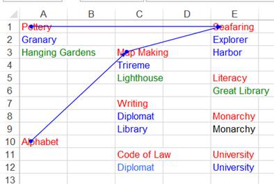
Figure 1

While the dated worksheet may be of limited value even to Civilization enthusiasts, the technique for creating the dependency tree is unique enough to be of value to Excel consumers. What makes it of value is that the game dependencies (in the context of work this would be the dependencies in the business model) had nothing to do with what Excel considers as dependencies! Consequently, to use Excel’s Trace Precedents feature I had to somehow map the model dependency into Excel formula dependencies.

For a version in a page by itself (i.e., not in a scrollable iframe as below) visit http://www.tushar-mehta.com/publish_train/xl_vba_cases/0908%20CIV%20game%20dependency%20tree.shtml
Tushar Mehta

Excel Advanced Filter

Excel supports two different ways to filter data that are in tabular format. Autofilter is a built-in capability driven via the user interface. As sophisticated as Autofilter has become in recent versions of Excel, no pre-defined setup can possibly cater to all the different questions that the consumer may want answered. These require a custom filter and Advanced Filter provides that capability. It is a data-driven mechanism that uses Excel formulas to extract specific information from the original data. For those who may have heard of SQL but have never been motivated to learn it, you can now leverage some of the power of SQL without learning a single word of SQL!

The layout of this document is as follows: 1) Introduction to the data set used in the examples, 2) Introduction to the Advanced Filter dialog box, 3) Filter using column headers, 4) Filter using Excel formulas, 5) Extract unique data, 6) Work with dynamic source data, and 7) Create a filter in a different worksheet or workbook.

For a version in a page by itself (i.e., not in a scrollable iframe as below) visit http://www.tushar-mehta.com/publish_train/data_analysis/06.shtml

Tushar Mehta

Freeze Panes and Split Panes

When working with a worksheet that contains a large number of rows and/or a large number of columns with row and column headers, it is very helpful to always view the headers no matter where one scrolls through the document.

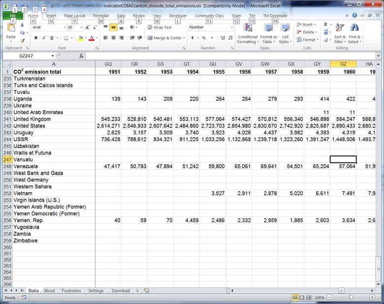
An example is shown below. The table lists the year-by-year carbon dioxide emissions by country (the data set comes from data download page at Gapminder – http://www.gapminder.org/data/). The current worksheet view shows data from the 1950s (columns GQ through GZ) and countries that are alphabetically towards the end of the list of countries (rows 235 through 259). At the same time, the column headers (row 1) and the row headers (column A) are still visible. This lets one quickly establish a context for the numbers. This is the result of using Excel’s Freeze Panes feature.

A complementary feature is called Split Panes. The key differences between freeze pane and split pane are the somewhat different behavior while scrolling and an easier way to adjust the panes, which, of course, comes with extra responsibility to manage the risk of accidental changes to the split panes configuration.

For a version in a page by itself (i.e., not in a scrollable iframe as below) visit http://www.tushar-mehta.com/publish_train/xl_vba_cases/0201%20split%20freeze%20pane.shtml

Tushar Mehta

TM Excel Dynamic Path Navigator

One of the features that consumers may find useful is retracing their path as they navigate through different workbooks, different sheets, and different windows. This navigation would be equivalent of a web browser’s Previous and Next feature. While Excel does not support this natively, the code in this note enables this capability.

For a version in a page by itself (i.e., not in a scrollable iframe as below) visit http://www.tushar-mehta.com/publish_train/xl_vba_cases/1110%20Workbook%20Navigation%20Retrace.shtml

Tushar Mehta

Copy Unique Values

One of the more frequent activities I perform is taking a list and extracting unique values as a seperate list.

The way to do this is long and stupid.
In Excel 2003 you select your range, go to the Data menu, Filter menu, select Advanced Filter. Select “Copy to another location”, tick “Unique records only”, then put a range in the “Copy To” box.
In Excel 2007 and above, it’s one less click. Go to the Data ribbon, from the Sort & Filter group click Advanced, then the same Advanced Filter window appears as Excel 2003.

Sick of this, a few years ago I wrote a macro to extract Unique Values, which worked so-so. My macro had minor issues that I could never really be bothered fixing, but it was miles better than trekking through those menus.
Fast forward to a couple of weeks ago and I lost my macro, somehow, which is disappointing, but it was buggy anyway, but I still wanted an easy way to extract unique values and I didn’t want to write the macro again.
It suddenly occurred to me that the same method of hitting shortcuts keys for paste values (alt, e, s, v) could be applied to copying unique values.

Here’s what I do:
Select the range I want to extract from
Hold down the Alt key
Press these keys in sequence: d, f, a, r, o, t
Release the Alt key
Select the range to paste the unique values to

It’s even possible to create a vba macro for this:
SendKeys "%(dfarot)"

Now, to train my muscle memory to type dfarot naturally…

Highlight row and column of active cell

By default, when the user selects a cell, Excel highlights the row and column by changing the color of the associated row and column headers. This tip shares multiple ways to highlight the row and column in more obvious ways as well as a way to highlight the cell in a specific column in the same row.


The emphasis is on the use of conditional formatting to accomplish the task. The minimal VBA code required to make it work is the same single executable statement for all of the different highlighting options!

For a version in a page by itself (i.e., not in a scrollable iframe as below) visit http://www.tushar-mehta.com/publish_train/xl_vba_cases/0121%20highlight%20row%20and%20col%20of%20selected%20cell.shtml

Tushar Mehta

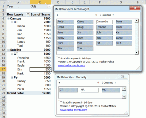
Introducing TM Retro Slicer

Those who have used a slicer in Excel 2010 slicer may want to see that capability in earlier versions of Excel. I like what Microsoft did with slicers in 2010 and have wanted to extend that capability backwards. For those who haven’t used a slicer, it is a filter on a particular pivot field shown as an independent object.

So, with TM Retro Slicer, one can create a slicer in any version of Excel from 2003 to 2010.

TM Retro Slicer works with versions of Excel from 2003 to 2010. Once enabled, a slicer will be visible on the worksheet.

Switching worksheets will hide the slicer and it will reappear when the worksheet is reactivated.

The slicer will remain across a workbook close and re-open.

For more on this shareware solution, please visit http://www.tushar-mehta.com/excel/software/retro_slicer/index.htm

Tushar Mehta