Analyze ‘free’ money

Recently, I received yet another promotion from yet another company offering me money at zero percent interest with the predictable asterisk next to the zero percent. Instead of just shredding the offer I decided to create a downloadable Excel template to analyze the offer, which was an interest-free 18 month loan for a 4% transaction fee with a minimum $10 fee.

Obviously, the transaction fee makes sure that the money is not ‘free.’ So, how does one calculate the cost of even the best emergency loans? I settled on an “effective interest rate.”
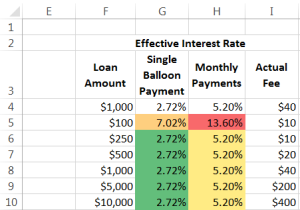
image001

For a version in a page by itself (i.e., not in a scrollable iframe as below) visit http://www.tushar-mehta.com/publish_train/xl_vba_cases/0920%20free%20money.shtml
Tushar Mehta

Excel Advanced Filter

Excel supports two different ways to filter data that are in tabular format. Autofilter is a built-in capability driven via the user interface. As sophisticated as Autofilter has become in recent versions of Excel, no pre-defined setup can possibly cater to all the different questions that the consumer may want answered. These require a custom filter and Advanced Filter provides that capability. It is a data-driven mechanism that uses Excel formulas to extract specific information from the original data. For those who may have heard of SQL but have never been motivated to learn it, you can now leverage some of the power of SQL without learning a single word of SQL!

The layout of this document is as follows: 1) Introduction to the data set used in the examples, 2) Introduction to the Advanced Filter dialog box, 3) Filter using column headers, 4) Filter using Excel formulas, 5) Extract unique data, 6) Work with dynamic source data, and 7) Create a filter in a different worksheet or workbook.

For a version in a page by itself (i.e., not in a scrollable iframe as below) visit http://www.tushar-mehta.com/publish_train/data_analysis/06.shtml

Tushar Mehta

Unicode and diacritic characters

The primary role of Excel is analysis and visualization of data, which put less emphasis on the use of special text characters. Nonetheless, there will always be some need for special characters, both Unicode characters and diacritics in Excel.

A diacritic in English is a glyph that modifies the sound of the character to which it is attached. Examples are naïve, résumé, and saké. In other fields, glyphs modify a letter to convey a specific meaning. Examples include:

· In Statistics the sample mean is denoted by x-bar (x̄) and the sample proportion by p-hat (p̂). Examples of Unicode characters are the population mean (the lowercase Greek letter mu, μ) and the population standard deviation (the lower case Greek letter sigma, σ).
· In Economics, profit is denoted by the Greek letter pi (π).
· In Mathematics, well, in Mathematics, there are a plethora of symbols including the capital sigma (Σ) for sum and ∫ for an integral.
· Currencies are denoted by symbols such as the US Dollar ($), the Euro (€), the Japanese Yen (¥), the Chinese Yuan (元), and the Indian Rupee (₹).

For a version in a page by itself (i.e., not in a scrollable iframe as below) visit http://www.tushar-mehta.com/publish_train/xl_vba_cases/0123%20Unicode%20and%20diacritics.shtml

Tushar Mehta

Freeze Panes and Split Panes

When working with a worksheet that contains a large number of rows and/or a large number of columns with row and column headers, it is very helpful to always view the headers no matter where one scrolls through the document.

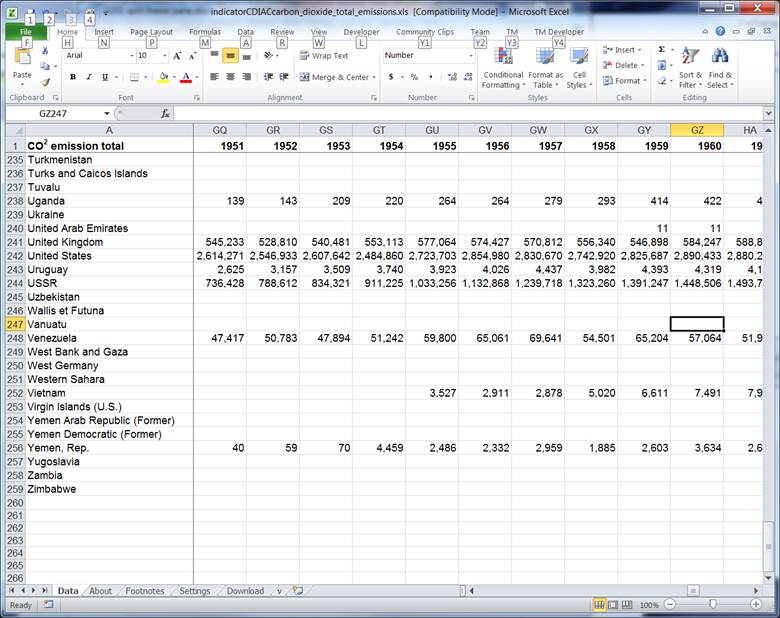
An example is shown below. The table lists the year-by-year carbon dioxide emissions by country (the data set comes from data download page at Gapminder – http://www.gapminder.org/data/). The current worksheet view shows data from the 1950s (columns GQ through GZ) and countries that are alphabetically towards the end of the list of countries (rows 235 through 259). At the same time, the column headers (row 1) and the row headers (column A) are still visible. This lets one quickly establish a context for the numbers. This is the result of using Excel’s Freeze Panes feature.

A complementary feature is called Split Panes. The key differences between freeze pane and split pane are the somewhat different behavior while scrolling and an easier way to adjust the panes, which, of course, comes with extra responsibility to manage the risk of accidental changes to the split panes configuration.

For a version in a page by itself (i.e., not in a scrollable iframe as below) visit http://www.tushar-mehta.com/publish_train/xl_vba_cases/0201%20split%20freeze%20pane.shtml

Tushar Mehta

Create a header cell with text separated by a diagonal line

In creating a table header that explains what the row and column values represent, a common approach is to use a cell with text separated by a diagonal line. This, first for me, video tutorial explains how.

For those who prefer a text explanation:

Format the cell “border” to add a diagonal from the left-top to the right-bottom (it’s one of the line choices in the Format Cells dialog box | Borders tab).

Then, type several spaces the literal Hours ALT+ENTER to create a newline in the text and then the literal Days.

Adjust the number of spaces before the literal Hours to get the desired effect.

An alternative, which is simple albeit crude, is to type Days space \ space Hours. {grin}

Tushar Mehta