Converting Numbers to Text

Posted on April 5, 2017 by Dick Kusleika

The difference between numbers and text is a concept that most Excel beginners don’t grasp. It’s not very intuitive. But to work with computers, you must think like a computer. To a computer, numbers are numbers and strings are strings regardless of what they look like.

How about an example. Let’s say you’re preparing data to fill out a form. Oh, I don’t know, just some random form like a Utah Excise Tax Return. You might have data that looks like this:

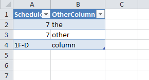
Experienced Excel users will immediately notice that the 7s are right justified, indicating they are numbers, and the 1F-D is left justified, indicating it’s a string. Everything in the Schedule column should be a string. The key test is: Do I perform mathematical operations on it. If so, it should be a number. If not, then it’s simply a label whose characters happen to be digits instead of letters.

Under most circumstances, this doesn’t really matter. Of course there’s no way I could stand to see two types of data in the same column, but normal people would have no problem with it. And the few that would have a problem would just change the alignment without changing the data type. There are, however, at least two situations where it can cause problems: long numbers and leading zeros. If you enter a 16-digit credit card number into Excel, it will truncate the last digit because Excel can only handle 15 digits of precision. If you enter a number like 04712495135 into a cell, the first zero will be gone as soon as you press enter.

The first thing you should do is to format your Table columns with the proper number format. That is, any columns that should be text should be formatted as text so the new entries are automatically considered text. It’s easy enough to do after the fact. And honestly I’m usually creating a table from data that already exists, so I can’t format a ListColumn before it exists. When you already have numbers in a text column, you need to do one extra step before you format (or after, it doesn’t matter the order).

Select the column and choose Text to Columns from the Data tab.

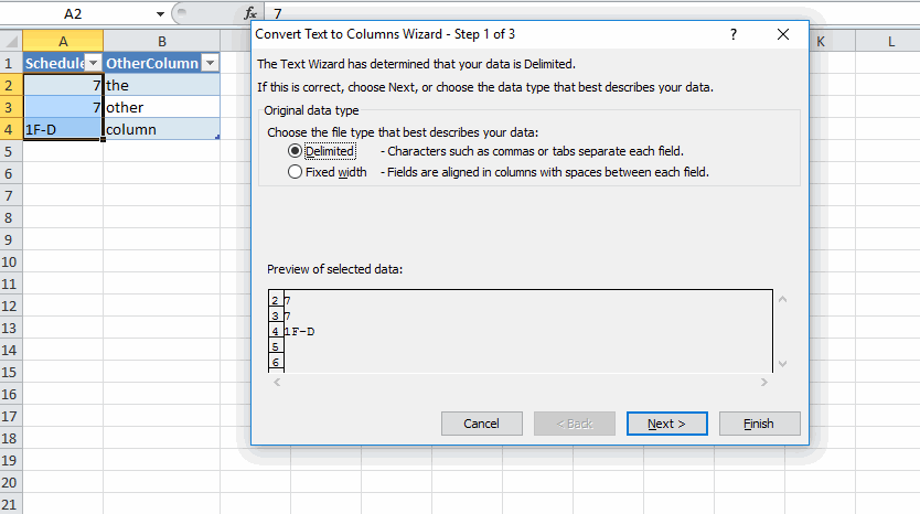
Choose delimited and click Next. Choose a delimiter that doesn’t exist anywhere in the data. I usually keep Tab checked for two reasons: 1) It’s pretty rare to have tabs in a cell and 2) Tab is the default and I’m speeding through this process pretty quickly (Alt+A, E, Alt+N, Alt+N, Alt+T, Alt+F).

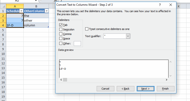
Finally, tell the wizard that the column is Text and click Finish.

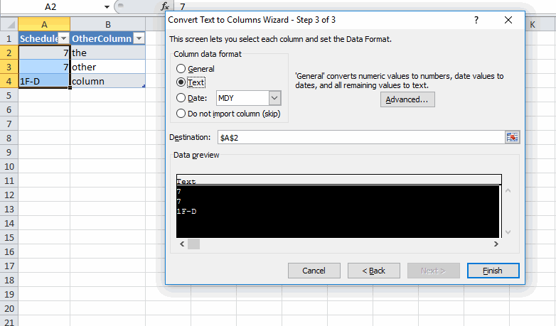
If you did it right (and haven’t changed your Excel options to hide certain errors), you’ll see some green triangles next to the “numbers” indicating that Excel is warning you that you have text that looks suspiciously like numbers.

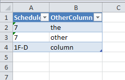
I’ve been working on an excise tax project lately that requires me to use other peoples workbooks and a lot of exported data. I run these steps several times a day so I decided it was time to automate it.

Public Sub ConvertColumnToText()

    Dim lo As ListObject
    Dim lc As ListColumn
    
    gclsAppEvents.AddLog "^+%t", "ConvertColumnToText"
    
    Set lo = ActiveCell.ListObject
    
    If Not lo Is Nothing Then
        Set lc = lo.ListColumns(ActiveCell.Column - lo.ListColumns(1).Range.Column + 1)
        With lc
            .DataBodyRange.TextToColumns .DataBodyRange, xlDelimited, xlTextQualifierDoubleQuote, False, False, , , , , , Array(1, 2)
            .DataBodyRange.NumberFormat = "@"
        End With
    End If

End Sub

Public Sub ConvertColumnToText()

Dim lo As ListObject

Dim lc As ListColumn

gclsAppEvents.AddLog "^+%t", "ConvertColumnToText"

Set lo = ActiveCell.ListObject

If Not lo Is Nothing Then

Set lc = lo.ListColumns(ActiveCell.Column - lo.ListColumns(1).Range.Column + 1)

With lc

.DataBodyRange.TextToColumns .DataBodyRange, xlDelimited, xlTextQualifierDoubleQuote, False, False, , , , , , Array(1, 2)

.DataBodyRange.NumberFormat = "@"

End With

End If

End Sub

KwikOpen Exclusions

Posted on March 21, 2017 by Dick Kusleika

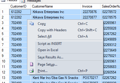
I use a product called SQL Prompt from Redgate in SSMS. Honestly I can’t image life without it. They added a new feature to the grid right-click menu called Open in Excel.

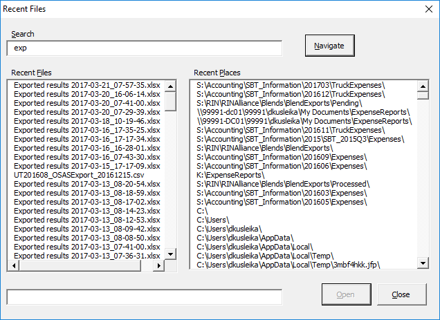
It’s very handy and definitely worth the trip over to my mouse. My only complaint about it is that it adds the resulting workbook to the MRU. That muddies up my KwikOpen Addin (original, update) particularly when I’m searching for “exported” or “results”.

I don’t think they should be adding that to the MRU and I’ve told them so. But in the meantime I’m going to exclude it from my list of files. Here’s the relevant part of the Fill method in the CRcntFiles class.

    For Each rf In Application.RecentFiles
        If Not rf.Path Like "*\Local\Temp\*Exported results *.xlsx" Then
            Set clsRcntFile = New CRcntFile
            clsRcntFile.FullName = rf.Path
            Me.Add clsRcntFile
        End If
    Next rf

For Each rf In Application.RecentFiles

If Not rf.Path Like "*\Local\Temp\*Exported results *.xlsx" Then

Set clsRcntFile = New CRcntFile

clsRcntFile.FullName = rf.Path

Me.Add clsRcntFile

End If

Next rf

I really need to build an exclusions interface where I can enter matching strings to exclude rather than putting it in the code. Someday.

Jumping to a PivotTable’s Source Data

Posted on March 2, 2017 by Dick Kusleika

I use Ctrl+[ all the time to go to the precedents of the ActiveCell. The SourceData for a PivotTable isn’t a precedent, but wouldn’t it be nice if there was a shortcut to go there? Yes, it would.

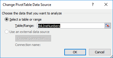
Until now, if I wanted to see the SourceData for a PivotTable, I would use Alt, J, T, I, D to activate the Ribbon control for changing the source data (PivotTable Tools – Options – Change Data Source – Change Data Source). That would open the Change PivotTable Data Source dialog. The focus on that dialog is a RefEdit control so Excel navigates to the data. I don’t actually want to change it, though, so I hit ESC and it takes me back to the PivotTable. But I make a note of where it is and I use Ctrl+G or simply navigate to where it is.

I decide to repurpose Ctrl+[ to do the deed.

Public Sub SelectPrecedents()
    
    gclsAppEvents.AddLog "^[", "SelectPrecedents"
    
    On Error Resume Next
        Selection.DirectPrecedents.Select
        Application.Goto ActiveCell.PivotTable.SourceData
        
End Sub

Public Sub SelectPrecedents()

gclsAppEvents.AddLog "^[", "SelectPrecedents"

On Error Resume Next

Selection.DirectPrecedents.Select

Application.Goto ActiveCell.PivotTable.SourceData

End Sub

First, I recorded a macro to see what happens when I press Ctrl+[. That became the first line after the error handler. Rather than doing a bunch of checking to see whether the ActiveCell was in a PivotTable, whether the PivotTable source was a Range, and a bunch of other stuff that I can’t even predict, I just attempt to Goto the SourceData. If it works, then it was possible. If there’s some reason I can’t, it just fails silently.

Displaying Formulas and Column Width

Posted on January 27, 2017 by Dick Kusleika

To display formulas in Excel, as opposed to displaying the formula results, you press the Ctrl+` key combination (that’s an accent grave and it’s to the left of the 1 on most US keyboards). When you do that, Excel helpfully increases the column width to show you more of the formula.

Excel increases the column width, but it doesn’t increase the ColumnWidth. That is, the ColumnWidth property is still the same even though you can see more characters than before. I’m not sure what exactly is changing here, but that’s not really the point of this post. The increase in width is about double. The percent of times that Excel makes the column wide enough to show me what I want to see is 0%.

If I have a 20 character formula, I’m probably not going to use Ctrl+` to check it out. It’s the longer formulas where I need to ensure consistency. I need to increase the column width even more, but that creates another problem. When I change the column width I also change the ColumnWidth. And when I go back to displaying formula results, my column width is now wider than it was. I’m working on a solution, but there’s a lot of moving pieces, so this isn’t fully baked yet.

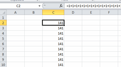
First I need to store the ColumnWidth before any changes. Then I need to increase the column width so I can see the whole formula. Then I need to set the ColumnWidth back to what it was. For the above formula, that’s pretty straightforward. It’s only about 150 characters. But the one below is about 280 characters and that strategy will make the column wider than the screen – no good.

Round one of my attempt to replace the Ctrl+` behavior is below.

Sub Macro1()

    Static dColWidth As Double
    Dim i As Long
    Dim ash As Worksheet
    Dim aw As Window 'activewindow
    Dim ec As Range 'activecell.entirecolumn
    
    Set ash = ActiveSheet
    Set aw = ActiveWindow
    Set ec = ActiveCell.EntireColumn
    
    'toggle
    aw.DisplayFormulas = Not aw.DisplayFormulas
    
    If aw.DisplayFormulas Then
        'store the old column width
        dColWidth = ec.ColumnWidth
        ec.AutoFit
        
        'Keep reducing the width by 10 until it fits on the screen
        For i = ec.ColumnWidth To ash.StandardWidth Step -10
            If ec.Column < aw.VisibleRange.Cells(aw.VisibleRange.Cells.Count).Column Then Exit For
            ec.ColumnWidth = i
        Next i
        
    Else
        'If the static variable loses scope, set
        'the column to the standard width
        If dColWidth > 0 Then
            ec.ColumnWidth = dColWidth
        Else
            ec.ColumnWidth = ash.StandardWidth
        End If
        
    End If
    
End Sub

Sub Macro1()

Static dColWidth As Double

Dim i As Long

Dim ash As Worksheet

Dim aw As Window 'activewindow

Dim ec As Range 'activecell.entirecolumn

Set ash = ActiveSheet

Set aw = ActiveWindow

Set ec = ActiveCell.EntireColumn

'toggle

aw.DisplayFormulas = Not aw.DisplayFormulas

If aw.DisplayFormulas Then

'store the old column width

dColWidth = ec.ColumnWidth

ec.AutoFit

'Keep reducing the width by 10 until it fits on the screen

For i = ec.ColumnWidth To ash.StandardWidth Step -10

If ec.Column < aw.VisibleRange.Cells(aw.VisibleRange.Cells.Count).Column Then Exit For

ec.ColumnWidth = i

Next i

Else

'If the static variable loses scope, set

'the column to the standard width

If dColWidth > 0 Then

ec.ColumnWidth = dColWidth

Else

ec.ColumnWidth = ash.StandardWidth

End If

End Sub

To combat really long formulas, I AutoFit the formula, then reduce the column width until it fits on the screen. It’s a bit more indirect than converting points to characters and all that funny business associated with ColumnWidth, but I like it. I haven’t tried to break it with hidden columns or anything like, so there’s probably some fragility there.

Five Minute Dashboards

Posted on January 25, 2017 by Dick Kusleika

Mike at Data Pig Technologies must have got some Christmas present he didn’t want because he’s having a giveaway.

The task is simple. Start with some prepared data and create a fully functional dashboard/report in 5 minutes or less.

To participate in this contest, you can submit a video of you building out a report or dashboard. All videos will be loaded to an official 5-Minute Challenge YouTube Playlist.

I think there are more prizes than there were a few days ago when I first read that post. Here’s a taste:

First Prize

XBox One

Second Prize

Fitbit Charge Heart Fitness Wristband

Third Prize

Amazon Fire Tablet

And much more. Visit http://datapigtechnologies.com/blog/index.php/new-contest-for-2017-the-excel-5-minute-challenge/ for all the details and updates.

Good VBA Dates and Bad Excel Dates

Posted on January 19, 2017 by Dick Kusleika

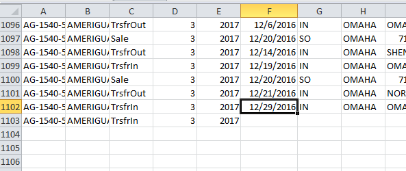
No, I’m not launching a match making service for Excel nerds. I’m talking about calendar dates. I was importing some data from a system that doesn’t seem to care what dates you might enter. Here’s the offender

TrsfrIn      03-2017  12/13/1206  IN    OMAHA   00243406         GL       440.0000        3.9400        1733.60     440.0000  GL

1	TrsfrIn 03-2017 12/13/1206 IN OMAHA 00243406 GL 440.0000 3.9400 1733.60 440.0000 GL

Instead of 2016, the user entered 1206. VBA doesn’t care.

?isdate("12/13/1206")
True

1 2	?isdate("12/13/1206") True

But Excel cares. As you know, Excel stores dates as the number of days since December 31, 1899. Anything before 1900-01-01 isn’t considered a date. The way this manifested was strange to me. I got the error (Application-defined or object-defined error) on this line

    rStart.Resize(UBound(vaWrite, 1), UBound(vaWrite, 2)).Value = vaWrite

1	rStart.Resize(UBound(vaWrite, 1), UBound(vaWrite, 2)).Value = vaWrite

When I filled the class, and specifically the TranDate property, no problem as VBA recognizes it as a date. When I fill the array vaWrite, no problem – the array contains text, numbers, and dates so it’s typed as a Variant. It’s only when I try to write it to a range that it complains. But why? I can type 12/13/1206 into a cell with no problem. It won’t recognize it as a date, but it doesn’t throw an error either.

A user (who is not me) got the error and clicked End. They’ve learned that clicking Debug only makes things worse – not that there are ever bugs in my code. When he clicked End, the code filled up the range all the way up to the bad date, line 1103.

That’s unexpected behavior. I would think the whole write operation would fail, but apparently not. The good news is that this partial writing of data led me to the root of the problem very quickly. The bad news is that the user was perfectly happy that clicking End produced data and he didn’t realize that the data wasn’t complete. He went on about his day until things just weren’t tying out properly. As much as I like the debugging help of a partial write, I think I would prefer if it didn’t write anything at all.

In any case, it’s an interesting insight into writing an array to a range all at once. It’s long known that filling an array and plopping it into a range is way faster than writing out cell-by-cell. But whatever you do in VBA to avoid looping, you’re not really avoiding looping. All you’re doing is moving the loop to a faster place. For instance, when you Join an array, something in VBA is looping, just not you. In this case, VBA is looping through vaWrite and filling up cells and it’s doing it faster than you or I could. The interesting thing to me is that it’s really a screen refresh that’s hiding the loop (maybe). As opposed to, say, VBA building a bunch of XML in the background and replacing part of the sheet.

But back to the error. Why an error anyway? As I said, I can type that non-date into Excel without error. I can even type that non-date in a cell and format the cell as a date without error. If I enter the formula =DATE(1206,12,13) in a cell, it returns 12/13/3106. Not a good result, but not an error either.

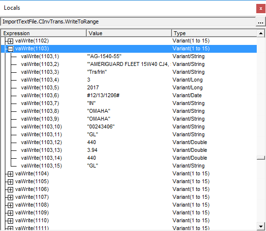
I think it all comes down to the fact that VBA has cast this data as a date and Excel won’t accept a date outside of its range. At least it won’t accept it from VBA. If I look at the locals window, I can see that my Variant Array has cast that value as a Variant/Date.

And this command in the Immediate Window fails with the same error as above

activecell.Value = dateserial(1206,12,13)

1	activecell.Value = dateserial(1206,12,13)

but if I override the cast by casting it as a String, it works

activecell.Value = cstr(dateserial(1206,12,13))

1	activecell.Value = cstr(dateserial(1206,12,13))

If you’ve followed me down this rabbit hole and are still reading, then may god have mercy on your soul. Here’s my fix

Public Sub FillFromRecordset(ByRef adRs As ADODB.Recordset, ByVal sItem As String, ByVal sDesc As String, ByVal sLoc As String)
    
    Dim dtTrans As Date
    
    With Me
        .ItemID = sItem
        .Description = Trim$(sDesc)
        .Location = Trim$(sLoc)
        .TranType = Trim$(Nz(adRs.Fields("TranType")))
        .Period = Split(adRs.Fields("PerYear"), "-")(0)
        .Year = Split(adRs.Fields("PerYear"), "-")(1)
        '.TranDate = Nz(adRs.Fields("TranDate"), 0)
        dtTrans = Nz(adRs.Fields("TranDate"), 0)
        
        If VBA.Year(dtTrans) < 1900 Then
            .TranDate = DateSerial(1900, Month(dtTrans), Day(dtTrans))
        Else
            .TranDate = dtTrans
        End If
        
        .Source = Trim$(Nz(adRs.Fields("Source")))
        .SourceID = Trim$(Nz(adRs.Fields("SourceID")))
        .RefNo = Trim$(Nz(adRs.Fields("RefNo")))
        .DefUnits = Trim$(Nz(adRs.Fields("DefUnits")))
        .DefQuantity = Nz(adRs.Fields("DefQuantity"), 0)
        .DefUnitCost = Nz(adRs.Fields("DefUnitCost"), 0)
        .Quantity = Nz(adRs.Fields("Quantity"), 0)
        .Units = Trim$(Nz(adRs.Fields("Units")))
    End With
    
End Sub

Public Sub FillFromRecordset(ByRef adRs As ADODB.Recordset, ByVal sItem As String, ByVal sDesc As String, ByVal sLoc As String)

Dim dtTrans As Date

With Me

.ItemID = sItem

.Description = Trim$(sDesc)

.Location = Trim$(sLoc)

.TranType = Trim$(Nz(adRs.Fields("TranType")))

.Period = Split(adRs.Fields("PerYear"), "-")(0)

.Year = Split(adRs.Fields("PerYear"), "-")(1)

'.TranDate = Nz(adRs.Fields("TranDate"), 0)

dtTrans = Nz(adRs.Fields("TranDate"), 0)

If VBA.Year(dtTrans) < 1900 Then

.TranDate = DateSerial(1900, Month(dtTrans), Day(dtTrans))

Else

.TranDate = dtTrans

End If

.Source = Trim$(Nz(adRs.Fields("Source")))

.SourceID = Trim$(Nz(adRs.Fields("SourceID")))

.RefNo = Trim$(Nz(adRs.Fields("RefNo")))

.DefUnits = Trim$(Nz(adRs.Fields("DefUnits")))

.DefQuantity = Nz(adRs.Fields("DefQuantity"), 0)

.DefUnitCost = Nz(adRs.Fields("DefUnitCost"), 0)

.Quantity = Nz(adRs.Fields("Quantity"), 0)

.Units = Trim$(Nz(adRs.Fields("Units")))

End With

End Sub

Instead of assigning the recordset date field to the property (I commented out that line), I assign it to a date variable and test the year. If the year is less than 1900, then I change it to 1900. I considered changing it to the current year, but I think having a different incorrect year that doesn’t cause an error is better than trying to guess what it should have been.

You might have noticed that I prefixed the Year function with VBA. I have a property in this class called Year, so when I try to use it, VBA thinks I’m referring the class property and not the VBA function. Prefixing the function call with the library name ensures that it uses the right one.

I wrote that Nz function back in 2007 but it’s been updated since. So here’s the new and improved version.

Function Nz(fldTest As ADODB.Field, _
    Optional vDefault As Variant) As Variant
   
    If IsNull(fldTest.Value) Then
        If IsMissing(vDefault) Then
            Select Case fldTest.Type
                Case adBSTR, adGUID, adChar, adWChar, adVarChar, adVarWChar
                    Nz = vbNullString
                Case Else
                    Nz = 0
            End Select
        Else
            Nz = vDefault
        End If
    Else
        If Not IsMissing(vDefault) Then
            If vDefault = 0 Then
                Nz = Replace(fldTest.Value, "*", "")
            Else
                Nz = fldTest.Value
            End If
        Else
            Nz = fldTest.Value
        End If
    End If
   
End Function

Function Nz(fldTest As ADODB.Field, _

Optional vDefault As Variant) As Variant

If IsNull(fldTest.Value) Then

If IsMissing(vDefault) Then

Select Case fldTest.Type

Case adBSTR, adGUID, adChar, adWChar, adVarChar, adVarWChar

Nz = vbNullString

Case Else

Nz = 0

End Select

Else

Nz = vDefault

End If

Else

If Not IsMissing(vDefault) Then

If vDefault = 0 Then

Nz = Replace(fldTest.Value, "*", "")

Else

Nz = fldTest.Value

End If

Else

Nz = fldTest.Value

End If

End Function

This is great example of a function that needs some comments.

Standing Desk Upgrade

Posted on January 17, 2017 by Dick Kusleika

I upgraded my standing desk from paper boxes to something a little fancier.

The three components are a monitor pole, a desk for the top of my desk, and a mat.

VIVO Dual Monitor Stand Up Desk Mount

Adjustable height standing desk.

Imprint CumulusPRO Anti-Fatigue Mat

I tried this laptop stand for my keyboard and mouse, but it was a little too unstable. A comment on Amazon said it was designed to hold seven pound laptops and a lightweight keyboard may not work as well. It wasn’t super wobbly, but enough that I didn’t like it.

Portable Laptop-Table-Stand with Mouse Pad

The whole getup ran about $170. Compare that to almost $400 for a real stand up desk without the floor mat.

VARIDESK Height Adjustable Standing Desk Black

The downside is that I have to raise and lower the monitors manually. I loosen the allen screw, slide the monitors down the pole, and re-tighten. That’s not as easy as it sounds. The weight of the monitors makes the sleeve that holds them bind against the pole. Sliding them down means first lifting them up to unbind the sleeve. If my desk backed up to a wall this would be impossible. You really have to be dedicated to frugality to want this set up.

The next step is moving the floor mat out of the way and moving the desktop desk over to my credenza. I don’t really have a lot of paper or other stuff on my credenza, so there’s plenty of room. But again, this is hardly a universally appropriate set up. If I decide I hate it, I’m only out $170, so there’s that.

Grouped Sheets Warning

Posted on January 12, 2017 by Dick Kusleika

We’ve all been there. I group a few sheets, change several things at once, and pat myself on the back for being so efficient. A few changes later, I realize that the sheets are still grouped and that I’m an idiot. I finally decided to do something about it and I happened on this old post from Contextures. Debra asks

What would you like Excel to do, to make grouped sheets more noticeable?

I’d like a warning, but I’d like it to be non-modal. That is, I don’t want it to interrupt me.

What about a hideous Ribbon tab that appears when you group sheets?

First, I used the CustomUI editor to add some XML to my workbook.

<customUI xmlns="http://schemas.microsoft.com/office/2009/07/customui" onLoad="GroupAlertRibbonLoad">
	<ribbon startFromScratch="false" >
		<tabs>
			<tab id="tabGroupAlert" label="Grouped Sheets Warning" getVisible="tabGroupAlert_GetVisible" >
				<group id="grpGroupAlert" label="Grouped Sheets Warning" >
					<button id="GA1" size="large" imageMso="ColorRed" />
					<button id="GA2" size="large" imageMso="ColorYellow" />
					<button id="GA3" size="large" imageMso="ColorRed" />
					<button id="GA4" size="large" imageMso="ColorYellow" />
					<button id="GA5" size="large" imageMso="ColorRed" />
					<button id="GA6" size="large" imageMso="ColorYellow" />
					<button id="GA7" size="large" imageMso="ColorRed" />
					<button id="GA8" size="large" imageMso="ColorYellow" />
					<button id="GA11" size="large" imageMso="ColorRed" />	
					<button id="GA12" size="large" imageMso="ColorYellow" />
					<button id="GA13" size="large" imageMso="ColorRed" />
					<button id="GA14" size="large" imageMso="ColorYellow" />	
					<button id="GA15" size="large" imageMso="ColorRed" />
					<button id="GA16" size="large" imageMso="ColorYellow" />	
					<button id="GA17" size="large" imageMso="ColorRed" />
					<button id="GA18" size="large" imageMso="ColorYellow" />	
					<button id="GA19" size="large" imageMso="ColorRed" />
					<button id="GA20" size="large" imageMso="ColorYellow" />	
					<button id="GA21" size="large" imageMso="ColorRed" />
					<button id="GA22" size="large" imageMso="ColorYellow" />	
					<button id="GA23" size="large" imageMso="ColorRed" />
					<button id="GA24" size="large" imageMso="ColorYellow" />	
					<button id="GA25" size="large" imageMso="ColorRed" />
					<button id="GA26" size="large" imageMso="ColorYellow" />	
				</group>
			</tab>
		</tabs>
	</ribbon>
</customUI>

<tabs>

</group>

</tab>

</tabs>

</ribbon>

</customUI>

It’s a couple dozen buttons with alternating colors. It appears whenever a sheet is activated and sheets are grouped. Here’s the code in a standard module

Public goRibbon As IRibbonUI

Private Const msMODULE As String = "MCallbacks()"

'Callback for customUI.onLoad
Sub GroupAlertRibbonLoad(ribbon As IRibbonUI)

    Set goRibbon = ribbon
    
End Sub

'Callback for tabGroupAlert getVisible
Sub tabGroupAlert_GetVisible(control As IRibbonControl, ByRef returnedVal)
    If Not ActiveWindow Is Nothing Then
        returnedVal = ActiveWindow.SelectedSheets.Count > 1
        If returnedVal Then
            goRibbon.ActivateTab "tabGroupAlert"
        End If
    End If
    
End Sub

Public goRibbon As IRibbonUI

Private Const msMODULE As String = "MCallbacks()"

'Callback for customUI.onLoad

Sub GroupAlertRibbonLoad(ribbon As IRibbonUI)

Set goRibbon = ribbon

End Sub

'Callback for tabGroupAlert getVisible

Sub tabGroupAlert_GetVisible(control As IRibbonControl, ByRef returnedVal)

If Not ActiveWindow Is Nothing Then

returnedVal = ActiveWindow.SelectedSheets.Count > 1

If returnedVal Then

goRibbon.ActivateTab "tabGroupAlert"

End If

End Sub

The onLoad procedure sets up a global Ribbon variable. The getVisible procedure controls whether you can see the custom tab. If the count of SelectedSheets is greater than one, returnedVal is set to True and that makes the tab visible. The If block shows the tab if it’s visible using the ActivateTab method.

In the ThisWorkbook module:

Private Sub Workbook_SheetActivate(ByVal Sh As Object)
    
    goRibbon.Invalidate
    
End Sub

Private Sub Workbook_SheetActivate(ByVal Sh As Object)

goRibbon.Invalidate

End Sub

When a sheet is activated, the Ribbon is invalidated and the getVisible procedure is forced to run again.

The next step would be to put this code in an add-in with a class module and application level events to monitor all workbooks.

You can download GroupSheetAlert.zip

Daily Dose of Excel

Haphazardly Posted Excel Information and Other Stuff

Author: Dick Kusleika

Converting Numbers to Text

KwikOpen Exclusions

Jumping to a PivotTable’s Source Data

Displaying Formulas and Column Width

Five Minute Dashboards

Good VBA Dates and Bad Excel Dates

Standing Desk Upgrade

Grouped Sheets Warning