Summing Times with a Floor

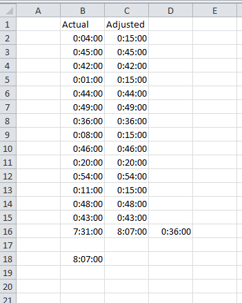
I have a list of times. Some of those times are less than 15 minutes and some are more. My billing floor is 15 minutes. That means that if a task takes me 4 minutes, I still bill 15.

In column C, I have this simple formula:

=MAX(TIME(0,15,0),B2)

That gives me the amount to bill; either 15 minutes or the actual time, whichever is greater. When I sum up that helper column, I get a total that’s 36 minutes more than the actual time. The challenge is to get rid of the helper column. And here’s the answer:

=SUM(B2:B15)+SUMPRODUCT((TIME(0,15,0)-B2:B15>0)*(TIME(0,15,0)-B2:B15))

The SUM simply sums the times and returns 7:31. The SUMPRODUCT section adds up the difference between 15 minutes and the actual time for all those times that are less than 15 minutes. If I use the Ctrl+= to calculate part of the formula, I get

=SUM(B2:B15)+SUMPRODUCT(({TRUE;FALSE;FALSE;TRUE;FALSE;FALSE;FALSE;TRUE;FALSE;FALSE;FALSE;TRUE;FALSE;FALSE})*({0.00763888888888889;-0.0208333333333333;-0.01875;0.00972222222222222;-0.0201388888888889;-0.0236111111111111;-0.0145833333333333;0.00486111111111111;-0.0215277777777778;-0.00347222222222222;-0.0270833333333333;0.00277777777777778;-0.0229166666666667;-0.0194444444444444}))

Yikes, that’s a long one. The first array is a TRUE if the value is less than 15 minutes and a FALSE if not. The second array is the actual difference between the time and 15 minutes. Recall that when TRUE and FALSE are forced to be a number (in this case, we force them to be a number by multiplying them), TRUE becomes 1 and FALSE becomes 0. When the two arrays are multiplied together

=SUM(B2:B15)+SUMPRODUCT({0.00763888888888889;0;0;0.00972222222222222;0;0;0;0.00486111111111111;0;0;0;0.00277777777777778;0;0})

Every value that was greater than zero gets multiplied by a 1, thereby returning itself. Every value that was less than zero gets multiplied by a 0, thereby returning zero. When you sum them all up, you get

=SUM(B2:B15)+0.025

And of course everyone knows that 2.5% of a day is the same as 36 minutes right? One of the bad things about using dates and times in the formula bar is that it converts them all to decimals. But .025 x 24 hours in a day x 60 minutes in an hour does equal 36 minutes. That gets added to the SUM of the actuals and Bob’s your uncle.

Is Patience a Virtue?

If you follow Nebraska football (and let’s be honest, who doesn’t?), then you know that Bo Pelini has been on and off the proverbial hot seat all year. Not surprisingly, Nebraska fans can’t see past the most recent game, so the seat gets hot after a loss and all is well after a win. I have been solidly in the pro-Bo camp. Not because I think he’s a great guy. He’s not. But we picked a horse and we need to stick with it to the end. You can’t go through all the hard times and then kick the guy out. That’s just stupid. We’ve been through six years of Pelini maturing as a coach, so let’s reap some of the benefits.

Then Iowa happened. There’s no shame in losing to Iowa; they’re a fundamentally solid team that makes very few mistakes. Nor is it “the way we lost” as has been said about Wisconsin and Georgia last year – horrifically embarrassing blowouts. What was noteworthy about yesterday was the way Pelini coached. A flea-flicker on the first play from scrimmage? A fake punt from deep in his own territory? It didn’t come off to me as a man trying to get that ninth win and keep his job. No, it seemed more like a man who already knew his fate and didn’t care about winning or losing. Following that was the post-game presser. Pelini said “chicken shit” on live TV, called out the referees (generally a no-no), and blamed the media for hurting the program. He came off like a colossal douche.

After all that, I still think we should keep him. I think he will be fired, I just don’t think he should be fired. (I have a different opinion about Offensive Coordinator Tim Beck, which you know if you’ve been within 100 yards of my house on game day.) For all the things I like about Bo Pelini, all I really want are national championships. Hell, I’d let Steve Spurrier coach here if he delivered that.

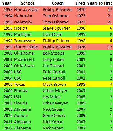
So the question becomes: Does firing Pelini get us closer or further away from a national championship? Yesterday DA and I did some back of the envelope analysis that I wanted to formalize today. Our hypothesis was that national championship coaches are hired, not built. Based on the last 20 AP national championships:

The green lines are coaches that won their first national championship within their first five years. Yellow is six to ten years. Red lines require patience. That makes a pretty good case for keeping the coaching carousel churning. That’s a lot of coaches winning national championships with athletes they didn’t necessarily recruit.

Conclusion: Hire a good recruiter, fire him after four years, then hire a good tactician. Or just hire Nick Saban – that works too.

On to some Excel stuff. The formula in E2 is {=MIN(IF($C$2:$C$21=C2,$A$2:$A$21,""))-D2}. It’s an array formula that finds the earliest year that coach won a national championship and subtracts the year he was hired.

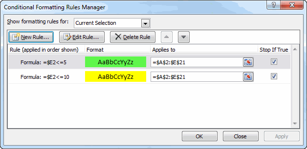
I wanted to use the fancy built-in conditional formatting to color the lines, but I couldn’t figure it out. There is a color scales option, but apparently it only applies to the cell and I couldn’t base the whole row’s color on column E. I had to roll my own color scales.

I changed the fill color of the whole range to red. That’s my default formatting. Now I can use conditional formatting to override that as the data warrants.

The “Stop if True” is important here so that future conditions aren’t evaluated.

Averaging Best 4 of 5 Golf Scores

Here’s part of a spreadsheet for a golf league.

The formula in AA is just an AVERAGE(), but the one in AB is a little more interesting. It looks like this:

{=IF(COUNT(B2:Z2)<5,AA2,(SUM((Z2:INDEX(A2:Z2,LARGE(COLUMN(A2:Z2)*(A2:Z2<>""),5))))-LARGE((Z2:INDEX(A2:Z2,LARGE(COLUMN(A2:Z2)*(A2:Z2<>""),5))),1))/4)}

This formula takes the last five scores, throws out the highest one, and averages the remaining four scores. If the player has less than five scores, it’s just a simple average. I did some similar calculations in Golf Handicap and Sum Last Three Golf Scores if you’re interested. Let’s break this one down.

Array Formula

First, this formula is an array formula. When you enter it correctly, using Ctrl+Shift+Enter rather than just Enter, Excel puts the curly braces around the formula. If you don’t enter it correctly, Excel will still usually return a result, just not the right result. So please enter it correctly. Stuff like this is why Enron doesn’t have a golf league anymore.

Some formulas act on numbers. 1+2 = 3 takes two numbers and adds them together. Array formulas act on arrays of numbers. {1,10,100}+{2,20,200} = {3,30,300}. As you can see, when the arrays are added, each element of the array is added to its brother and the result isn’t a number, it’s an array of numbers. If you want to see a cleaner example of an array formula and how they work, go read Anatomy of an Array Formula.

The IF Part

{=IF(COUNT(B2:Z2)<5,AA2,*Some Array Stuff*)}

The IF part is pretty straight forward. The COUNT function returns how many numbers are in the range to see if there are enough scores. If there are, do the array magic. If there aren't, get the average that we've computed in AA2.

The SUM Part

(SUM(*Stuff that returns an array*)-LARGE(*Stuff that returns an array*,1)/4

Remember when I said that adding arrays returns an array. The same is true for multiplication. The purpose of an array formula is to return an array into a function that does something with an array. We don't want to get an array back from our formula, we want to get an array to plug into the SUM function so that we can add it up and get one number back.

In this part of the formula, we're summing up the array, subtracting out the 1st largest value (LARGE(x,1) returns the largest value in x, while LARGE(x,3) returns the third largest value.), and finally dividing the whole mess by 4 to get an average.

The INDEX Part

Z2:INDEX(A2:Z2,*Some array stuff that returns a column number*)

Cell references that span more than one cell look like B2:Z2, with a colon separating the first cell in the range with the last cell in the range. What you may not know is that Excel doesn't really care which order they're in. To Excel, Z2:B2 is the same as B2:Z2. Go try it. Go type =SUM(Z2:B2) in a worksheet and see what happens.

In this part of the formula, we're starting with Z2, then a colon. The INDEX function is going to return a cell reference that makes up the second part of our multi-cell range. For instance, on line 3 in the above screen shot, the INDEX function is going to return K3, so that when Excel evaluates the formula in AB3, it will reduce this part to Z3:K3 and then convert that to K3:Z3. K3:Z3 happens to be the range that covers Andrew's last five scores.

With INDEX, you supply a range and a number that says which cell in that range you want. In our example, we're supplying the range A3:Z3 (the entirety of the scores) and we're doing some calculations that return which cell in A3:Z3 we want to be the Z3's partner.

The LARGE Part

LARGE(*the array stuff*,5)

In The SUM part, we talked about how LARGE works because we were trying to find the largest number in an array to get rid of. Here we're using LARGE in a different part of the formula. We're finding the 5th largest value in some array. Why fifth? Because we want five golf scores. This is the part that, in line 3, helps us find K3 so we can sum up K3:Z3.

The array that we're getting the 5th largest value from is an array of column numbers that have non-blank cells. Of all the cells on line 3 between A and Z, K3 is the fifth largest column number (K=11 if column letters were actually numbers) if you only consider cells that aren't blanks. N3 would be the fourth largest and P3 the second largest, to name a few.

The Array Part

COLUMN(A2:Z2)*(A2:Z2<>"")

Finally the good part. This is the part where we multiply two arrays together and the part that makes this formula an array formula rather than the normal kind. We've kind of worked from the outside in on this formula, but I'm going to walk back from the inside out so we don't lose perspective on this part.

The array part returns an array of column numbers. That goes into the LARGE function so we can find the fifth largest column number that has a value. That cell gets married to Z3 to make a multi-cell range. The range gets put into a SUM function that adds up the five scores in the range.

You may notice that the array part is repeated in the formula. It's in the SUM part so we can get to the five values. It's also in the LARGE part so we can pick out the largest of those five values to discard.

I mentioned earlier that we can multiply arrays and get an array in return. We're multiplying two arrays that each have 26 elements (A-Z is 26).

COLUMN(A3:Z3)*(A3:Z3<>"")

As arrays, the above looks like this:

{1,2,3,4,5,6,7,8,9,10,11,12,13,14,15,16,17,18,19,20,21,22,23,24,25,26}*{TRUE,TRUE,TRUE,TRUE,TRUE,TRUE,FALSE,FALSE,TRUE,TRUE,TRUE,FALSE,FALSE,TRUE,TRUE,TRUE,TRUE,FALSE,FALSE,FALSE,FALSE,FALSE,FALSE,FALSE,FALSE,FALSE}

The COLUMN function returns the column number for the range, 1 to 26 in this case. The second array is created by comparing each cell in A3:Z3 to an empty string, thereby testing whether the cell is empty. If it's not equal to an empty string, that element of the array gets a TRUE. If it is empty, it gets a FALSE. We end up with 26 TRUEs and FALSEs telling us which columns have values.

Now here's the magic. When you do math on a TRUE or FALSE, it converts into a number; TRUE becomes 1 and FALSE becomes 0. When we multiply each element of the arrays to each other, remembering how TRUEs and FALSEs are treated, we get

{1,2,3,4,5,6,0,0,9,10,11,0,0,14,15,16,17,0,0,0,0,0,0,0,0,0}

Every column that had a value gets the column number. Every column that had no value gets a zero. We have a 26 element array with column numbers and zeros. This array gets jammed into a LARGE function that returns the fifth largest value. What's the fifth largest value in this array? It's 11.

The 11 gets jammed into and INDEX function to return the 11th cell of A3:Z3, which is K3.

K3 gets tacked onto Z3 to make Z3:K3 and that gets converted to K3:Z3.

K3:Z3 gets jammed into a SUM function and returns 40, the sum of the last five scores. Elsewhere, K3:Z3 gets jammed into a LARGE(x,1) function to return the largest value in K3:Z3, or 14.

We take the sum, 40, subtract the large, 14, and get 26. Divide 26 by 4 and we get 6.5, the number in AB3.

And that's it. Now you know about array formulas, INDEX, LARGE, COUNT, and COLUMN. I assume you already knew about IF and SUM. Do you get how it works? OK smart guy. What do you need to change to get the best 4 out of 6?
Handicap History

Back in 2005, I created a spreadsheet to calculate my USGA handicap and I’ve been using it ever since (175 scores posted). It calculates my current handicap but doesn’t give me any historical information. Until now.

GHIN calculates handicaps on a schedule, not in real time. That means many of the handicaps on my spreadsheet aren’t official. They do that so that one score doesn’t swing the calculation too much. By calculating approximately monthly, they give you a chance to post a few scores between calculations. Here’s what my spreadsheet looks like today:

The formulas up to column J are the same as they were in 2005. I’ve added formulas in K through O.

K181: =SUMPRODUCT(((H162:H181+(ROW(H162:H181)/100000))<=SMALL(H162:H181+(ROW(H162:H181)/100000),10))*(H162:H181))

The part that says +(ROW(H162:H181)/100000) is used to add a small number so that I can break ties but won't affect the score. Otherwise it's summing up the 10 smallest of the last 20. I started 20 rows down so I wouldn't have to mess with less than 20 scores. That's too much work for not enough payoff.

L181: =SUMPRODUCT(--((H162:H181+(ROW(H162:H181)/100000))<=SMALL(H162:H181+(ROW(H162:H181)/100000),10)))

I don't know why I wrote this one - it's always 10. Except that sometimes it was 11 before I added the +ROW stuff to break ties. It's principally the same formula as the previous one except for the last part. And it includes the double-negation to coerce the Trues and Falses into numbers.

M181: =TRUNC(K181/L181*0.96,1)

Divide one by t'other and take 96%.

N181: =IF((M181+(ROW(M181)/100000))=MIN(IF(((YEAR($D$27:$D$181)=YEAR(D181))*($M$27:$M$181))=0,"",($M$27:$M$181+(ROW($M$27:$M$181)/100000)))),M181,NA())
O181: =IF((M181+(ROW(M181)/100000))=MAX((YEAR($D$27:$D$181)=YEAR(D181))*(($M$27:$M$181+(ROW($M$27:$M$181)/100000)))),M181,NA())

Once I got that part done, the data was begging to be graphed. Once on a chart, I could see that I needed some Min's and Max's to clutter it up. These last two formulas compute the minimum and maximum indexes by year and return that value on the row where it exists. If it doesn't exist on a particular row, it returns NA() so it doesn't show up on the chart.

To make the chart, I selected all the data from D:O and created an XY chart. Then I deleted all the series that I didn't want. Sorry for the 2003isness of the chart. Some of the steps I took to create this chart are:

  • CumIndex: Remove markers, make Olive Green line, add Polynomial2 trendline
  • Trendline: Make 25% grey
  • Major Gridlines: Make 25% grey
  • Min: Remove lines, make makers green, make data labels = Y values, put data labels on bottom
  • Max: Remove lines, make makers red, make data labels = Y values, put data labels on top
  • Y axis: Make minimum of 4 and maximum of 16 to get rid of some white space
  • X axis: Adjust min and max to tighten it up
  • Plot area: Remove fill

Oh, how I pine for the days of a 7.5 handicap index. The season in Nebraska ends November 15, so I have a little more than two months to get that down. I'd like to get it down to, at most, an 8.0 by then.

You can download Handicap2.zip

Working with the MAXIF() and LARGEIF() functions

Oh, Wait! Excel doesn’t have those functions. We’ll have to roll our own. We’re going to use the Double Unary tip found here. In Excel, 1*TRUE = 1, 0+TRUE = 1, TRUE^1 = 1, and minus-minus TRUE (–TRUE, the double unary) = 1. It’s two sign changes, and thought to be the best way to turn an array of TRUE/FALSE into ones/zeros. Multiplying an array of parameters by an array of ones and zeros leaves only the TRUE parameters non-zero.

Back to our list of the 122 major teams in professional sports, the Boss has decided that sorting by name length, then alphabetically, isn’t going to do. He wants it by name length by stadium size. So, thanks to Wikipedia, your data looks like this, Column(F) is arena size:

  D E F
1 Anaheim Ducks 13 17,174
2 Arizona Cardinals 17 63,400
3 Arizona Diamondbacks 20 48,633
4 Atlanta Braves 14 50,097
5 Atlanta Falcons 15 71,228
6 Atlanta Hawks 13 18,729
7 Baltimore Orioles 17 45,363
8 Baltimore Ravens 16 71,008
9 Boston Bruins 13 17,565
10 Boston Celtics 14 18,624

Using fzz’s comment about the ROW() function, we’ll sort the length by G1=LARGE($E$1:$E$122,ROWS($G$1:$G1)) filled down. The table looks much like before:

  D E F G
1 Anaheim Ducks 13 17,174 29
2 Arizona Cardinals 17 63,400 22
3 Arizona Diamondbacks 20 48,633 22
4 Atlanta Braves 14 50,097 22
5 Atlanta Falcons 15 71,228 21
6 Atlanta Hawks 13 18,729 21
7 Baltimore Orioles 17 45,363 21
8 Baltimore Ravens 16 71,008 20
9 Boston Bruins 13 17,565 20
10 Boston Celtics 14 18,624 20

We know there are only three teams of name length 22. A formula – -($E$1:$E$122=22), using the double unary operation, gives us an array of 119 zeros, and just 3 ones that line up on 22. If we multiply that array by the array of arena capacities (F1:F122) we have 119 multiplications by zero, and three multiplications by 1. A MAX() function or an equivalent LARGE(,1) function on that array product returns the capacity of largest stadium hosting a team name 22 letters long. Those equations formulas, array entered, would look like this:

  • {=LARGE(- -($E$1:$E$122=22)*$F$1:$F$122,1)}
  • {=MAX(- -($E$1:$E$122=22)*$F$1:$F$122)}

We want to modify those for different teams. Changing the =22 to =$G1 is a start, and we’ve gone about as far as we can with our ‘MAXIF().’ It’s going to return the same thing three times. A scheme using COUNTIF() starting from the top and working down will improve the ‘LARGEIF()’. Using mixed references, $G$1:$G1 will grow as we fill down. COUNTIF($G$1:$G2,$G2) will only count one 22, COUNTIF($G$1:$G3,$G3) will count two 22s, and COUNTIF($G$1:$G4,$G4) will count 3, and that’s all there are. This array-entered equationformula then, filled down, is ‘LARGEIF()’:

  • {=LARGE(- -($E$1:$E$122=$G1)*$F$1:$F$122,COUNTIF($G$1:$G1,$G1))}

In I1 filldown =MATCH(H1,$F$1:$F$122,0) and in J1 filldown =INDEX(D:D,I1). Your table should look like this:

  D E F G H I J K
1 Anaheim Ducks 13 17,174 29 45,389 52 Los Angeles Angels of Anaheim  
2 Arizona Cardinals 17 63,400 22 19,980 95 Portland Trail Blazers  
3 Arizona Diamondbacks 20 48,633 22 19,356 63 Minnesota Timberwolves  
4 Atlanta Braves 14 50,097 22 18,144 30 Columbus Blue Jackets  
5 Atlanta Falcons 15 71,228 21 43,651 89 Philadelphia Phillies  
6 Atlanta Hawks 13 18,729 21 19,596 42 Golden State Warriors  
7 Baltimore Orioles 17 45,363 21 18,203 83 Oklahoma City Thunder  
8 Baltimore Ravens 16 71,008 20 68,756 69 New England Patriots  
9 Boston Bruins 13 17,565 20 67,164 49 Jacksonville Jaguars  
10 Boston Celtics 14 18,624 20 65,857 108 Tampa Bay Buccaneers  

Column(I) shows the indices reordered by size of the arena.

There are some problems with this approach. It only works with positive numbers, such as our capacities. Negative numbers will be less than a FALSE, and a zero will be returned in their place. And if ever capacities are equal, it will always return only the first (same old problem). Nicely here, hockey and basketball held in the same arena draw to different capacity. The file is available at http://wl.filegenie.com/~JMOprof/LargeIF.xls

…mrt
©¿©¬