This nifty formula is from Jim Young. Like me, Jim plays in a golf league that computes your handicap based on your last three scores. Unlike me, Jim is in a league whose administrator has a computer, not just an email machine. It would be straight forward to sum the last three scores of all the golfers, except that all the golfers don’t show up every week. Gaps in the scores make it a little trickier. Take this seven week scoring sheet
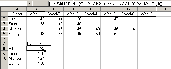
Not every golfer has a score for every week. To sum the last three scores, Jim uses an array formula. Let’s look at it from the inside out.
COLUMN(A2:H2)*(A2:H2<>"") evaluates to
{1,2,3,4,0,6,0,0}
The column number for columns with scores and zeros for columns with no scores
LARGE({1,2,3,4,0,6,0,0},3) evaluates to
3
The third largest number in the array (the first is 6, the second is 4). Column three contains the first column that we want to include in the sum. The INDEX function returns that range (C2 in this case) and our SUM function now looks like
=SUM(H2:C2)
This appears to be summing too many columns. But we know that the extra columns are blank because we filtered those out earlier. Summing blank cells has no effect on the sum because they are treated as zero. We get the sum of the last three scores and continue with our handicap calculation.
For more on array formulas, see Anatomy of an Array Formula.
Thanks for the formula Jim, and keep them coming.
Sorry, but I can’t believe any spreadsheet that has a bunch of golf scores that are under 50 for 9 holes. On behalf of the hackers of the world, I accuse these guys of score manipulation. Fredo is especially egregious in this regard. Winter rules, anyone? :-)
I am trying to work out a formula so that i can show in a cell, +3 or -3 for a golf score. The -3 is no problem, but I dont know how to show the positive sign for the positive numbers. How do you do this??
Please help, I am trying to work out a formula to create my golf handicap in Australia and do this in excel plus record and adjust the four players handicaps as we go along. I will be using a palm reader so do not want to use macros.
I am sure some one would have already done much homework in this regard and do not want to re create wheel….
Regards
Peter
It is out of my knowledge about the Excel…nice job!!!
To Jeff (post #2):
Format | Cells (ctrl 1)
first tab (Number)
in Category, select Custom
in the next box, type:
+0;0;0
OK
The formula gives me a #NUM! value for the COLUMN command in Excel v. 11.6355
I have tried this formula and cannot get it to work
because I get an error #NUM!. when I work with the formula the problem seems to be in the Column portion
it does not find the range start of C2.
Help from someone would be appreciated.
Roger: Make sure you’re entering the formula with Control+Shift+Enter, not just Enter.
I can make this work with the scores running horrizontally as in the example
how do you do the same thing with scores running down verticall?
If your scores in column I, then try this
Using this same logic how would you remove the lowest score (min) and the highest score (max)… and based on this idea say you had 5 scores and wanted the use this same logic.
This takes the sum of the last five and subtracts the largest score and the fifth largest score.
Thank you so much for posting this! I wanted to get this on Google Sheets so we could (gasp) maybe go paperless in our league, but could not get the array formula to work…my current fix is probably best described as brute force – a bunch of nested if statements to deal with people who miss weeks (if count =3, get average, if not expand range by 1 and test again). if they miss more than 4 weeks in a 7 week period issues will arise, but if they miss that much, are they really part of the league?
As I wrote this, I realize that I have never attempted to use Microsoft’s online Excel…maybe this is a good excuse to do so!
thank you.
Your formula helped greatly for finding the sum of the numbers from right to left. How would I adjust the formula to sum the data from left to right; to find the sum of the first 4 columns skipping zeros?
=IF(COUNT(A2:BF2)<4,"NA",SUM(BF2:INDEX(A2:BF2,LARGE(COLUMN(A2:BF2)*(A2:BF2″”),4))))
Mark: When you use
SMALL, you have to get rid of zeros in an array formula (and you need SMALL for this)=SUM(A2:INDEX(A2:H2,SMALL(IF(A2:H2="","",COLUMN(A2:H2)*(A2:H2<>"")),4)+1))