Jeff here, again. PivotTables again. Sorry ’bout that.
snb posted a very concise bit of code to unwind crosstabs over at Unpivot by SQL and so I got to wondering how my much longer routine handled in comparison.
My approach used SQL and lots of Union All statements to do the trick. And lots and lots of code. Whereas snb uses arrays to unwind the crosstab, which is fine so long as you don’t run out of worksheet to post the resulting flat-file in. Which is going to be the case 99.999999% of the time. And frankly, crosstabs in the other 0.000001% of cases deserve to be stuck as crosstabs.
At the same time, I thought I’d also test a previous approach of mine that uses the Multiple Consolidation trick that Mike Alexander outlines at Transposing a Dataset with a PivotTable. This approach:
- copies the specific contiguous or non-contiguous columns of data that the user want to turn into a flat file to a new sheet.
- concatenates all the columns on the left into one column, while putting the pipe character ‘|’ between each field so that later we can split these apart into separate columns again.
- creates a pivot table out of this using Excel’s ‘Multiple Consolidation Ranges’ option. Normally this type of pivot table is used for combining data on different sheets, but it has the side benefit of taking horizontal data and providing a vertical extract once you double click on the Grand Total field. This is also known as a ‘Reverse Pivot’.
- splits our pipe-delimited column back into seperate columns, using Excel’s Text-to-Column funcionality.
snb’s approach
snbs’ code for a dataset with two non-pivot fields down the left looked like this:
|
1 2 3 4 5 6 7 8 9 10 11 12 13 14 15 16 17 18 |
Sub M_snb() sn = Cells(1).CurrentRegion x = Cells(1).CurrentRegion.Rows(1).SpecialCells(2).Count y = UBound(sn, 2) - x ReDim sp(1 To x * (UBound(sn) - 1), 1 To 4) For j = 1 To UBound(sp) m = (j - 1) Mod (UBound(sn) - 1) + 2 n = (j - 1) \ (UBound(sn) - 1) + y + 1 sp(j, 1) = sn(m, 1) sp(j, 2) = sn(m, 2) sp(j, 3) = sn(1, n) sp(j, 4) = sn(m, n) Next Cells(20, 1).Resize(UBound(sp), UBound(sp, 2)) = sp End Sub |
…which I’m sure you’ll all agree falls somewhere on the spectrum between good looking and positivity anorexic. So I put a bit of meat on it’s bones so that it prompts you for ranges and handles any sized cross-tab:
|
1 2 3 4 5 6 7 8 9 10 11 12 13 14 15 16 17 18 19 20 21 22 23 24 25 26 27 28 29 30 31 32 33 34 35 36 37 38 39 40 41 42 43 44 45 46 47 48 49 50 51 52 53 54 55 56 57 58 59 60 61 62 63 64 65 66 67 68 69 70 71 72 73 74 75 76 77 78 79 80 81 82 83 84 85 86 87 88 89 90 91 92 93 94 95 96 97 98 99 100 101 102 103 104 105 106 107 108 109 110 111 112 113 114 115 116 117 118 119 120 121 122 123 |
Sub UnPivot_snb() Dim varSource As Variant Dim j As Long Dim m As Long Dim n As Long Dim i As Long Dim varOutput As Variant Dim rngCrossTab As Range Dim rngLeftHeaders As Range Dim rngRightHeaders As Range 'Identify where the ENTIRE crosstab table is If rngCrossTab Is Nothing Then On Error Resume Next Set rngCrossTab = Application.InputBox( _ Title:="Please select the ENTIRE crosstab", _ prompt:="Please select the ENTIRE crosstab that you want to turn into a flat file", _ Type:=8, Default:=Selection.CurrentRegion.Address) If Err.Number <> 0 Then On Error GoTo errhandler Err.Raise 999 Else: On Error GoTo errhandler End If rngCrossTab.Parent.Activate rngCrossTab.Cells(1, 1).Select 'Returns them to the top left of the source table for convenience End If 'Identify range containing columns of interest running down the table If rngLeftHeaders Is Nothing Then On Error Resume Next Set rngLeftHeaders = Application.InputBox( _ Title:="Select the column HEADERS from the LEFT of the table that WON'T be aggregated", _ prompt:="Select the column HEADERS from the LEFT of the table that won't be aggregated", _ Default:=Selection.Address, Type:=8) If Err.Number <> 0 Then On Error GoTo errhandler Err.Raise 999 Else: On Error GoTo errhandler End If Set rngLeftHeaders = rngLeftHeaders.Resize(1, rngLeftHeaders.Columns.Count) 'just in case they selected the entire column rngLeftHeaders.Cells(1, rngLeftHeaders.Columns.Count + 1).Select 'Returns them to the right of the range they just selected End If If rngRightHeaders Is Nothing Then 'Identify range containing data and cross-tab headers running across the table On Error Resume Next Set rngRightHeaders = Application.InputBox( _ Title:="Select the column HEADERS from the RIGHT of the table that WILL be aggregated", _ prompt:="Select the column HEADERS from the RIGHT of the table that WILL be aggregated", _ Default:=Selection.Address, _ Type:=8) If Err.Number <> 0 Then On Error GoTo errhandler Err.Raise 999 Else: On Error GoTo errhandler End If Set rngRightHeaders = rngRightHeaders.Resize(1, rngRightHeaders.Columns.Count) 'just in case they selected the entire column rngCrossTab.Cells(1, 1).Select 'Returns them to the top left of the source table for convenience End If If strCrosstabName = "" Then 'Get the field name for the columns being consolidated e.g. 'Country' or 'Project'. note that reserved SQL words like 'Date' cannot be used strCrosstabName = Application.InputBox( _ Title:="What name do you want to give the data field being aggregated?", _ prompt:="What name do you want to give the data field being aggregated? e.g. 'Date', 'Country', etc.", _ Default:="Date", _ Type:=2) If strCrosstabName = "False" Then Err.Raise 999 End If timetaken = Now() varSource = rngCrossTab lRightColumns = rngRightHeaders.Columns.Count lLeftColumns = UBound(varSource, 2) - lRightColumns ReDim varOutput(1 To lRightColumns * (UBound(varSource) - 1), 1 To lLeftColumns + 2) For j = 1 To UBound(varOutput) m = (j - 1) Mod (UBound(varSource) - 1) + 2 n = (j - 1) \ (UBound(varSource) - 1) + lLeftColumns + 1 varOutput(j, lLeftColumns + 1) = varSource(1, n) varOutput(j, lLeftColumns + 2) = varSource(m, n) For i = 1 To lLeftColumns varOutput(j, i) = varSource(m, i) Next i Next j Worksheets.Add With Cells(1, 1) .Resize(, lLeftColumns).Value = rngLeftHeaders.Value .Offset(, lLeftColumns).Value = strCrosstabName .Offset(, lLeftColumns + 1).Value = "Value" .Offset(1, 0).Resize(UBound(varOutput), UBound(varOutput, 2)) = varOutput End With timetaken = timetaken - Now() Debug.Print "UnPivot - snb: " & Now() & " Time Taken: " & Format(timetaken, "HH:MM:SS") errhandler: If Err.Number <> 0 Then Dim strErrMsg As String Select Case Err.Number Case 999: 'User pushed cancel. Do nothing Case 998 'Worksheet does not have enough rows to hold flat file strErrMsg = "Oops, there's not enough rows in the worsheet to hold a flatfile of all the data you have selected. " strErrMsg = strErrMsg & vbNewLine & vbNewLine strErrMsg = strErrMsg & "Your dataset will take up " & Format(rngRightHeaders.CurrentRegion.Count, "#,##0") & " rows of data " strErrMsg = strErrMsg & "but your worksheet only allows " & Format(Application.Range("A:A").Count, "#,##0") & " rows of data. " strErrMsg = strErrMsg & vbNewLine & vbNewLine MsgBox strErrMsg Case Else MsgBox Err.Description, vbCritical, "UnPivot_snb" End Select End If End Sub |
Talk about yo-yo dieting!
Multiple Consolidation Trick approach
And here’s my code that uses the Multiple Consolidation trick:
|
1 2 3 4 5 6 7 8 9 10 11 12 13 14 15 16 17 18 19 20 21 22 23 24 25 26 27 28 29 30 31 32 33 34 35 36 37 38 39 40 41 42 43 44 45 46 47 48 49 50 51 52 53 54 55 56 57 58 59 60 61 62 63 64 65 66 67 68 69 70 71 72 73 74 75 76 77 78 79 80 81 82 83 84 85 86 87 88 89 90 91 92 93 94 95 96 97 98 99 100 101 102 103 104 105 106 107 108 109 110 111 112 113 114 115 116 117 118 119 120 121 122 123 124 125 126 127 128 129 130 131 132 133 134 135 136 137 138 139 140 141 142 143 144 145 146 147 148 149 150 151 152 153 154 155 156 157 158 159 160 161 162 163 164 165 166 167 168 169 170 171 172 173 174 175 176 177 178 179 180 181 182 183 184 185 186 187 188 189 190 191 192 193 194 195 196 197 198 199 200 201 202 203 204 205 206 207 208 209 210 211 212 213 214 215 216 217 218 219 220 221 222 223 224 225 226 227 228 229 230 231 232 233 234 235 236 237 238 239 240 241 242 243 244 245 246 247 248 249 250 |
Option Explicit Sub CallUnPivotByConsolidation() Call UnPivotByConsolidation End Sub Function UnPivotByConsolidation( _ Optional rngCrossTab As Range, _ Optional rngLeftHeaders As Range, _ Optional rngRightHeaders As Range, _ Optional strCrosstabName As String) As Boolean Dim wksTempCrosstab As Worksheet Dim wksInitial As Worksheet Dim strConcat As String Dim strCell As String Dim strFormula As String Dim iCount As Integer Dim iColumns As Integer Dim iRows As Integer Dim rngInputData As Range Dim wksPT As Worksheet Dim wksFlatFile As Worksheet Dim pc As PivotCache Dim pt As PivotTable Dim rngKeyFormula As Range Dim rngRowHeaders As Range Dim rngPT_GrandTotal As Range, rngPTData As Range Dim lPT_Rows As Long Dim iPT_Columns As Integer Dim iKeyColumns As Integer Dim varRowHeadings As Variant ''''''''''''''''''''''''''''''''''''''''''''''''''''''''''''''''''''''''''''' 'Part one: ' 'Code prompts user to select contiguous or non-contiguous columns of data ' 'from a crosstab table, and writes it to a new sheet in a contiguous range. ' ''''''''''''''''''''''''''''''''''''''''''''''''''''''''''''''''''''''''''''' Set wksInitial = ActiveSheet 'Identify where the ENTIRE crosstab table is If rngCrossTab Is Nothing Then On Error Resume Next Set rngCrossTab = Application.InputBox( _ Title:="Please select the ENTIRE crosstab", _ prompt:="Please select the ENTIRE crosstab that you want to turn into a flat file", _ Type:=8, Default:=Selection.CurrentRegion.Address) If Err.Number <> 0 Then On Error GoTo errhandler Err.Raise 999 Else: On Error GoTo errhandler End If rngCrossTab.Parent.Activate rngCrossTab.Cells(1, 1).Select 'Returns them to the top left of the source table for convenience End If 'Identify range containing columns of interest running down the table If rngLeftHeaders Is Nothing Then On Error Resume Next Set rngLeftHeaders = Application.InputBox( _ Title:="Select the column HEADERS from the LEFT of the table that WON'T be aggregated", _ prompt:="Select the column HEADERS from the LEFT of the table that won't be aggregated", _ Default:=Selection.Address, Type:=8) If Err.Number <> 0 Then On Error GoTo errhandler Err.Raise 999 Else: On Error GoTo errhandler End If Set rngLeftHeaders = Intersect(rngLeftHeaders.EntireColumn, rngCrossTab) rngLeftHeaders.Cells(1, rngLeftHeaders.Columns.Count + 1).Select 'Returns them to the right of the range they just selected End If If rngRightHeaders Is Nothing Then 'Identify range containing data and cross-tab headers running across the table On Error Resume Next Set rngRightHeaders = Application.InputBox( _ Title:="Select the column HEADERS from the RIGHT of the table that WILL be aggregated", _ prompt:="Select the column HEADERS from the RIGHT of the table that WILL be aggregated", _ Default:=Selection.Address, _ Type:=8) If Err.Number <> 0 Then On Error GoTo errhandler Err.Raise 999 Else: On Error GoTo errhandler End If Set rngRightHeaders = Intersect(rngRightHeaders.EntireColumn, rngCrossTab) rngCrossTab.Cells(1, 1).Select 'Returns them to the top left of the source table for convenience End If If strCrosstabName = "" Then 'Get the field name for the columns being consolidated e.g. 'Country' or 'Project'. note that reserved SQL words like 'Date' cannot be used strCrosstabName = Application.InputBox( _ Title:="What name do you want to give the data field being aggregated?", _ prompt:="What name do you want to give the data field being aggregated? e.g. 'Date', 'Country', etc.", _ Default:="Date", _ Type:=2) If strCrosstabName = "False" Then Err.Raise 999 End If With Application .ScreenUpdating = False .DisplayAlerts = False End With 'Set up a temp worksheet to house our crosstab data For Each wksTempCrosstab In ActiveWorkbook.Worksheets If wksTempCrosstab.Name = "TempCrosstab" Then wksTempCrosstab.Delete Next Set wksTempCrosstab = Worksheets.Add wksTempCrosstab.Name = "TempCrosstab" 'Copy data to the temp worksheet "TempCrosstab" rngLeftHeaders.Copy wksTempCrosstab.[A1] Set rngLeftHeaders = wksTempCrosstab.[A1].CurrentRegion rngLeftHeaders.Name = "TempCrosstab!appRowFields" rngRightHeaders.Copy wksTempCrosstab.[A1].Offset(0, rngLeftHeaders.Columns.Count) Set rngRightHeaders = wksTempCrosstab.[A1].Resize(rngRightHeaders.Rows.Count, rngRightHeaders.Columns.Count) rngRightHeaders.Name = "TempCrosstab!appCrosstabFields" 'Work out if the worksheet has enough rows to fit a crosstab in If rngRightHeaders.CurrentRegion.Count > Columns(1).Rows.Count Then Err.Raise 998 varRowHeadings = rngLeftHeaders.Value ''''''''''''''''''''''''''''''''''''''''''''''''''''''''''''''''''''''''''''' 'Part Two: ' 'Construct a new pipe-delimited column out of the columns that run down the ' 'left of the crosstab, and then delete the original columns used to do this ' ''''''''''''''''''''''''''''''''''''''''''''''''''''''''''''''''''''''''''''' strFormula = "=RC[1]" strConcat = "&""|""&" iColumns = Range("TempCrosstab!appRowFields").Columns.Count For iCount = 2 To iColumns strCell = "RC[" & iCount & "]" strFormula = strFormula & strConcat & strCell Next iCount With Worksheets("TempCrosstab") .Columns("A:A").Insert Shift:=xlToRight iRows = Intersect(Worksheets("TempCrosstab").Columns(2), Worksheets("TempCrosstab").UsedRange).Rows.Count .Range("A2:A" & iRows).FormulaR1C1 = strFormula .Range("A2:A" & iRows).Value = .Range("A2:A" & iRows).Value .Range("appRowFields").Delete Shift:=xlToLeft End With Names("TempCrosstab!appRowFields").Delete ''''''''''''''''''''''''''''''''''''''''''''''''''''''''''''''''''''''''''''''''' 'Part Three: ' 'Use data to create a pivot table using "Multiple Consolidation Ranges" option, ' 'which has the side benefit of providing a vertical extract once you double ' 'click on the Grand Total field ' ''''''''''''''''''''''''''''''''''''''''''''''''''''''''''''''''''''''''''''''''' Set rngInputData = Worksheets("TempCrosstab").[A2].CurrentRegion rngInputData.Name = "SourceData" 'Find out the number of columns contained within the primary key iKeyColumns = Len([SourceData].Cells(2, 1).Value) - Len(Replace([SourceData].Cells(2, 1).Value, "|", "")) + 1 ' Create the intermediate pivot from which to extract flat file Set pc = ActiveWorkbook.PivotCaches.Add(SourceType:=xlConsolidation, SourceData:=Array("=sourcedata", "Item1")) Set wksPT = Worksheets.Add Set pt = wksPT.PivotTables.Add(PivotCache:=pc, TableDestination:=[A3]) ' Get address of PT Total field, then double click it to get underlying records Set rngPTData = pt.DataBodyRange lPT_Rows = rngPTData.Rows.Count iPT_Columns = rngPTData.Columns.Count Set rngPT_GrandTotal = rngPTData.Cells(1).Offset(lPT_Rows - 1, iPT_Columns - 1) rngPTData.Cells(1).Offset(lPT_Rows - 1, iPT_Columns - 1).Select Selection.ShowDetail = True Set wksFlatFile = ActiveSheet ' Delete current "Flat_File" worksheet if it exists, name current sheet "Flat_File" On Error Resume Next Sheets("Flat_File").Delete On Error GoTo 0 wksFlatFile.Name = "Flat_File" ' Delete unneeded column and the now-unneeded TempCrosstab and wksPT worksheets Columns(4).Delete Shift:=xlToLeft wksPT.Delete Worksheets("TempCrosstab").Delete '''''''''''''''''''''''''''''''''''''''''''''''''''''''''''''''''''''''''''' 'Part Four: ' 'split our pipe-delimited column back into seperate columns, using Excel's ' 'Text-to-Column funcionality. ' '''''''''''''''''''''''''''''''''''''''''''''''''''''''''''''''''''''''''''' Set rngKeyFormula = Worksheets("Flat_File").Range("A2") rngKeyFormula.Name = "appKeyFormula" 'Find out the number of columns contained within the primary key iKeyColumns = Len([appKeyFormula].Cells(2, 1).Value) - Len(Replace([appKeyFormula].Cells(2, 1).Value, "|", "")) + 1 'Insert columns to the left that we will unpack the Unique Key to [B1].Resize(, iKeyColumns).EntireColumn.Insert 'Split the Unique Key column into its constituent parts, 'using Excel's Text-to-Columns functionality Worksheets("Flat_File").Columns("A:A").Select Selection.TextToColumns Destination:=Range("b1"), DataType:=xlDelimited, _ ConsecutiveDelimiter:=False, Other:=True, OtherChar:="|" 'Delete old composite key, add original column headers [A1].EntireColumn.Delete Set rngRowHeaders = [A1].Resize(1, iKeyColumns) rngRowHeaders.Value = varRowHeadings 'Add new column header with crosstab data name [A1].Offset(0, iKeyColumns).Value = strCrosstabName Selection.CurrentRegion.Columns.AutoFit Worksheets("Flat_File").Select errhandler: If Err.Number <> 0 Then Dim strErrMsg As String Select Case Err.Number Case 999: 'User pushed cancel. Do nothing Case 998 'Worksheet does not have enough rows to hold flat file strErrMsg = "Oops, there's not enough rows in the worsheet to hold a flatfile of all the data you have selected. " strErrMsg = strErrMsg & vbNewLine & vbNewLine strErrMsg = strErrMsg & "Your dataset will take up " & Format(rngRightHeaders.CurrentRegion.Count, "#,##0") & " rows of data " strErrMsg = strErrMsg & "but your worksheet only allows " & Format(Application.Range("A:A").Count, "#,##0") & " rows of data. " strErrMsg = strErrMsg & vbNewLine & vbNewLine MsgBox strErrMsg Case Else MsgBox Err.Description, vbCritical, "UnPivotByConsolidation" End Select End If With Application .ScreenUpdating = True .DisplayAlerts = True End With End Function |
The SQL appoach is the same as I published here.
And the winner is…
…snb. By a long shot. With the ever-so-slight caveat that you’re crosstabs are not so stupidly fat that the resulting flat file exceeds the number of rows in Excel.
Here’s how things stacked up on a 53 Column x 2146 Row crosstab, which gives a 117,738 row flat-file:
| Approach | Time (M:SS) |
|---|---|
| snb | 0:01 |
| UnPivotByConsolidation | 0:04 |
| UnPivotBySQL | 0:14 |
And here’s how things stacked up on a 53 Columns x 19,780 Row crosstab, giving a 1,048,340 row flat-file (i.e. practically the biggest sized crosstab that you can unwind):
| Approach | Time (M:SS) |
|---|---|
| snb | 0:19 |
| UnPivotByConsolidation | 0:42 |
| UnPivotBySQL | 2:17 |
So there you have it. Use snb’s code. Unless you have no choice but to use my longer, slower SQL approach.
—Update 26 November 2013—
It was remiss of me not to mention the Data Normalizer routine in Doug Glancy’s great yoursumbuddy blog, which is just about as fast as snb’s approach below. Go check it out, and subscribe to Doug’s blog while you’re there if you haven’t already.
—
If you don’t want the hassle of working out which to use, here’s a routine that uses snb’s if possible, and otherwise uses mine:
|
1 2 3 4 5 6 7 8 9 10 11 12 13 14 15 16 17 18 19 20 21 22 23 24 25 26 27 28 29 30 31 32 33 34 35 36 37 38 39 40 41 42 43 44 45 46 47 48 49 50 51 52 53 54 55 56 57 58 59 60 61 62 63 64 65 66 67 68 69 70 71 72 73 74 75 76 77 78 79 80 81 82 83 84 85 86 87 88 89 90 91 92 93 94 95 96 97 98 99 100 101 102 103 104 105 106 107 108 109 110 111 112 113 114 115 116 117 118 119 120 121 122 123 124 125 126 127 128 129 130 131 132 133 134 135 136 137 138 139 140 141 142 143 144 145 146 147 148 149 150 151 152 153 154 155 156 157 158 159 160 161 162 163 164 165 166 167 168 169 170 171 172 173 174 175 176 177 178 179 180 181 182 183 184 185 186 187 188 189 190 191 192 193 194 195 196 197 198 199 200 201 202 203 204 205 206 207 208 209 210 211 212 213 214 215 216 217 218 219 220 221 222 223 224 225 226 227 228 229 230 231 232 233 234 235 236 237 238 239 240 241 242 243 244 245 246 247 248 249 250 251 252 253 254 255 256 257 258 259 260 261 262 263 264 265 266 267 268 269 270 271 272 273 274 275 276 277 278 279 280 281 282 283 284 285 286 287 288 289 290 291 292 293 294 295 296 297 298 299 300 301 302 303 304 305 306 307 308 309 310 311 312 313 314 315 316 317 318 319 320 321 322 323 324 325 326 327 328 329 330 331 332 333 334 335 336 337 338 339 340 341 342 343 344 345 346 347 348 349 350 351 352 353 354 355 356 357 358 359 360 361 362 363 364 365 366 367 368 369 370 371 372 373 374 375 376 377 378 379 380 381 382 383 384 385 386 387 388 389 390 391 392 393 394 395 396 397 398 399 400 401 402 403 404 405 406 407 |
Option Explicit Sub Call_UnPivot() UnPivot End Sub Function unpivot(Optional rngCrossTab As Range, _ Optional rngLeftHeaders As Range, _ Optional rngRightHeaders As Range, _ Optional strCrosstabName As String, _ Optional rngOutput As Range, _ Optional bSkipBlanks As Boolean = False) As Boolean ' Desc: Turns a crosstab file into a flatfile using array manipulation. ' If the resulting flat file will be too long to fit in the worksheet, ' the routine uses SQL and lots of 'UNION ALL' statements to do the ' equivalent of the 'UNPfaddIVOT' command in SQL Server (which is not available ' in Excel)and writes the result directly to a PivotTable ' Base code for the SQL UnPivot derived from from Fazza at MR EXCEL forum: ' http://www.mrexcel.com/forum/showthread.php?315768-Creating-a-pivot-table-with-multiple-sheets ' The Microsoft JET/ACE Database engine has a hard limit of 50 'UNION ALL' clauses, but Fazza's ' code gets around this by creating sublocks of up to 25 SELECT/UNION ALL statements, and ' then unioning these. ' Programmer: Jeff Weir ' Contact: weir.jeff@gmail.com ' Name/Version: Date: Ini: Modification: ' UnPivot V1 20131122 JSW Original Development ' Inputs: Range of the entile crosstab ' Range of columns down the left that WON'T be normalized ' Range of columns down the right that WILL be normalize ' String containing the name to give columns that will be normalized ' Outputs: A pivottable of the input data on a new worksheet. ' Example: ' It takes a crosstabulated table that looks like this: ' Country Sector 1990 1991 ... 2009 ' ============================================================================= ' Australia Energy 290,872 296,887 ... 417,355 ' New Zealand Energy 23,915 25,738 ... 31,361 ' United States Energy 5,254,607 5,357,253 ... 5,751,106 ' Australia Manufacturing 35,648 35,207 ... 44,514 ' New Zealand Manufacturing 4,389 4,845 ... 4,907 ' United States Manufacturing 852,424 837,828 ... 735,902 ' Australia Transport 62,121 61,504 ... 83,645 ' New Zealand Transport 8,679 8,696 ... 13,783 ' United States Transport 1,484,909 1,447,234 ... 1,722,501 ' And it returns the same data in a recordset organised like this: ' Country Sector Year Value ' ==================================================== ' Australia Energy 1990 290,872 ' New Zealand Energy 1990 23,915 ' United States Energy 1990 5,254,607 ' Australia Manufacturing 1990 35,648 ' New Zealand Manufacturing 1990 4,389 ' United States Manufacturing 1990 852,424 ' Australia Transport 1990 62,121 ' New Zealand Transport 1990 8,679 ' United States Transport 1990 1,484,909 ' Australia Energy 1991 296,887 ' New Zealand Energy 1991 25,738 ' United States Energy 1991 5,357,253 ' Australia Manufacturing 1991 35,207 ' New Zealand Manufacturing 1991 4,845 ' United States Manufacturing 1991 837,828 ' Australia Transport 1991 61,504 ' New Zealand Transport 1991 8,696 ' United States Transport 1991 1,447,234 ' ... ... ... ... ' ... ... ... ... ' ... ... ... ... ' Australia Energy 2009 417,355 ' New Zealand Energy 2009 31,361 ' United States Energy 2009 5,751,106 ' Australia Manufacturing 2009 44,514 ' New Zealand Manufacturing 2009 4,907 ' United States Manufacturing 2009 735,902 ' Australia Transport 2009 83,645 ' New Zealand Transport 2009 13,783 ' United States Transport 2009 1,722,501 Const lngMAX_UNIONS As Long = 25 Dim varSource As Variant Dim varOutput As Variant Dim lLeftColumns As Long Dim lRightColumns As Long Dim i As Long Dim j As Long Dim m As Long Dim n As Long Dim lOutputRows As Long Dim arSQL() As String Dim arTemp() As String Dim sTempFilePath As String Dim objPivotCache As PivotCache Dim objRS As Object Dim oConn As Object Dim sConnection As String Dim wks As Worksheet Dim wksNew As Worksheet Dim cell As Range Dim strLeftHeaders As String Dim wksSource As Worksheet Dim pt As PivotTable Dim rngCurrentHeader As Range Dim timetaken As Date Dim strMsg As String Dim varAnswer As Variant Const Success As Boolean = True Const Failure As Boolean = False unpivot = Failure 'Identify where the ENTIRE crosstab table is If rngCrossTab Is Nothing Then Application.ScreenUpdating = True On Error Resume Next Set rngCrossTab = Application.InputBox( _ Title:="Please select the ENTIRE crosstab", _ Prompt:="Please select the ENTIRE crosstab that you want to turn into a flat file", _ Type:=8, Default:=Selection.CurrentRegion.Address) If Err.Number <> 0 Then On Error GoTo ErrHandler Err.Raise 999 Else: On Error GoTo ErrHandler End If rngCrossTab.Parent.Activate rngCrossTab.Cells(1, 1).Select 'Returns them to the top left of the source table for convenience End If 'Identify range containing columns of interest running down the table If rngLeftHeaders Is Nothing Then On Error Resume Next Set rngLeftHeaders = Application.InputBox( _ Title:="Select the column HEADERS from the LEFT of the table that WON'T be aggregated", _ Prompt:="Select the column HEADERS from the LEFT of the table that won't be aggregated", _ Default:=Selection.Address, Type:=8) If Err.Number <> 0 Then On Error GoTo ErrHandler Err.Raise 999 Else: On Error GoTo ErrHandler End If Set rngLeftHeaders = rngLeftHeaders.Resize(1, rngLeftHeaders.Columns.Count) 'just in case they selected the entire column Range(rngLeftHeaders.Cells(1, rngLeftHeaders.Columns.Count + 1), rngLeftHeaders.Cells(1, rngLeftHeaders.Columns.Count + 1).End(xlToRight)).Select 'Returns them to the right of the range they just selected End If If rngRightHeaders Is Nothing Then 'Identify range containing data and cross-tab headers running across the table On Error Resume Next Set rngRightHeaders = Application.InputBox( _ Title:="Select the column HEADERS from the RIGHT of the table that WILL be aggregated", _ Prompt:="Select the column HEADERS from the RIGHT of the table that WILL be aggregated", _ Default:=Selection.Address, _ Type:=8) If Err.Number <> 0 Then On Error GoTo ErrHandler Err.Raise 999 Else: On Error GoTo ErrHandler End If Set rngRightHeaders = rngRightHeaders.Resize(1, rngRightHeaders.Columns.Count) 'just in case they selected the entire column rngCrossTab.Cells(1, 1).Select 'Returns them to the top left of the source table for convenience End If If strCrosstabName = "" Then 'Get the field name for the columns being consolidated e.g. 'Country' or 'Project'. note that reserved SQL words like 'Date' cannot be used strCrosstabName = Application.InputBox( _ Title:="What name do you want to give the data field being aggregated?", _ Prompt:="What name do you want to give the data field being aggregated? e.g. 'Date', 'Country', etc.", _ Default:="Date", _ Type:=2) If strCrosstabName = "False" Then Err.Raise 999 End If If rngOutput Is Nothing Then 'Identify range containing data and cross-tab headers running across the table On Error Resume Next Set rngOutput = Application.InputBox( _ Title:="Where do you want to output the data", _ Prompt:="Select the top left cell where you want the transformed data to be output", _ Default:=Cells(ActiveSheet.UsedRange.row, ActiveSheet.UsedRange.Columns.Count + ActiveSheet.UsedRange.Column + 1).Address, _ Type:=8) If Err.Number <> 0 Then On Error GoTo ErrHandler Err.Raise 999 Else: On Error GoTo ErrHandler End If End If timetaken = Now() Application.ScreenUpdating = False 'Work out if the worksheet has enough rows to fit a crosstab in If Intersect(rngRightHeaders.EntireColumn, rngCrossTab).Cells.Count <= Columns(1).Rows.Count Then 'Resulting flat file will fit on the sheet, so use array manipulation. varSource = rngCrossTab lRightColumns = rngRightHeaders.Columns.Count lLeftColumns = UBound(varSource, 2) - lRightColumns If Not bSkipBlanks Then ReDim varOutput(1 To lRightColumns * (UBound(varSource) - 1), 1 To lLeftColumns + 2) Else lOutputRows = Application.WorksheetFunction.CountA(Intersect([appRightHeaders].EntireColumn, rngCrossTab)) - [appRightHeaders].Cells.Count ReDim varOutput(1 To lOutputRows, 1 To lLeftColumns + 2) End If If Not bSkipBlanks Then For j = 1 To UBound(varOutput) m = (j - 1) Mod (UBound(varSource) - 1) + 2 n = (j - 1) \ (UBound(varSource) - 1) + lLeftColumns + 1 varOutput(j, lLeftColumns + 1) = varSource(1, n) varOutput(j, lLeftColumns + 2) = varSource(m, n) For i = 1 To lLeftColumns varOutput(j, i) = varSource(m, i) Next i Next j Else lOutputRows = 1 For j = 1 To Intersect([appRightHeaders].EntireColumn, rngCrossTab).Cells.Count - [appRightHeaders].Cells.Count m = (j - 1) Mod (UBound(varSource) - 1) + 2 n = (j - 1) \ (UBound(varSource) - 1) + lLeftColumns + 1 If Not IsEmpty(varSource(m, n)) Then varOutput(lOutputRows, lLeftColumns + 1) = varSource(1, n) varOutput(lOutputRows, lLeftColumns + 2) = varSource(m, n) For i = 1 To lLeftColumns varOutput(lOutputRows, i) = varSource(m, i) Next i lOutputRows = lOutputRows + 1 End If Next j End If With rngOutput .Resize(, lLeftColumns).Value = rngLeftHeaders.Value .Offset(, lLeftColumns).Value = strCrosstabName .Offset(, lLeftColumns + 1).Value = "Quantity" .Offset(1, 0).Resize(UBound(varOutput), UBound(varOutput, 2)) = varOutput End With Else 'Resulting flat file will fit on the sheet, so use SQL and write result directly to a pivot strMsg = " I can't turn this crosstab into a flat file, because the crosstab is so large that" strMsg = strMsg & " the resulting flat file will be too big to fit in a worksheet. " strMsg = strMsg & vbNewLine & vbNewLine strMsg = strMsg & " However, I can still turn this information directly into a PivotTable if you want." strMsg = strMsg & " Note that this might take several minutes. Do you wish to proceed?" varAnswer = MsgBox(Prompt:=strMsg, Buttons:=vbOK + vbCancel + vbCritical, Title:="Crosstab too large!") If varAnswer <> 6 Then Err.Raise 999 If ActiveWorkbook.Path <> "" Then 'can only proceed if the workbook has been saved somewhere Set wksSource = rngLeftHeaders.Parent 'Build part of SQL Statement that deals with 'static' columns i.e. the ones down the left For Each cell In rngLeftHeaders 'For some reason this approach doesn't like columns with numeric headers. ' My solution in the below line is to prefix any numeric characters with ' an apostrophe to render them non-numeric, and restore them back to numeric ' after the query has run If IsNumeric(cell) Or IsDate(cell) Then cell.Value = "'" & cell.Value strLeftHeaders = strLeftHeaders & "[" & cell.Value & "], " Next cell ReDim arTemp(1 To lngMAX_UNIONS) 'currently 25 as per declaration at top of module ReDim arSQL(1 To (rngRightHeaders.Count - 1) \ lngMAX_UNIONS + 1) For i = LBound(arSQL) To UBound(arSQL) - 1 For j = LBound(arTemp) To UBound(arTemp) Set rngCurrentHeader = rngRightHeaders(1, (i - 1) * lngMAX_UNIONS + j) arTemp(j) = "SELECT " & strLeftHeaders & "[" & rngCurrentHeader.Value & "] AS Total, '" & rngCurrentHeader.Value & "' AS [" & strCrosstabName & "] FROM [" & rngCurrentHeader.Parent.Name & "$" & Replace(rngCrossTab.Address, "$", "") & "]" If IsNumeric(rngCurrentHeader) Or IsDate(rngCurrentHeader) Then rngCurrentHeader.Value = "'" & rngCurrentHeader.Value 'As per above, can't have numeric headers Next j arSQL(i) = "(" & Join$(arTemp, vbCr & "UNION ALL ") & ")" Next i ReDim arTemp(1 To rngRightHeaders.Count - (i - 1) * lngMAX_UNIONS) For j = LBound(arTemp) To UBound(arTemp) Set rngCurrentHeader = rngRightHeaders(1, (i - 1) * lngMAX_UNIONS + j) arTemp(j) = "SELECT " & strLeftHeaders & "[" & rngCurrentHeader.Value & "] AS Total, '" & rngCurrentHeader.Value & "' AS [" & strCrosstabName & "] FROM [" & rngCurrentHeader.Parent.Name & "$" & Replace(rngCrossTab.Address, "$", "") & "]" If IsNumeric(rngCurrentHeader) Or IsDate(rngCurrentHeader) Then rngCurrentHeader.Value = "'" & rngCurrentHeader.Value 'As per above, can't have numeric headers Next j arSQL(i) = "(" & Join$(arTemp, vbCr & "UNION ALL ") & ")" 'Debug.Print Join$(arSQL, vbCr & "UNION ALL" & vbCr) ''''''''''''''''''''''''''''''''''''''''''''''''''''''''''''''''' ' When using ADO with Excel data, there is a documented bug ' causing a memory leak unless the data is in a different ' workbook from the ADO workbook. ' http://support.microsoft.com/kb/319998 ' So the work-around is to save a temp version somewhere else, ' then pull the data from the temp version, then delete the ' temp copy sTempFilePath = ActiveWorkbook.Path sTempFilePath = sTempFilePath & "\" & "TempFile_" & Format(Time(), "hhmmss") & ".xlsm" ActiveWorkbook.SaveCopyAs sTempFilePath ''''''''''''''''''''''''''''''''''''''''''''''''''''''''''''''''' If Application.Version >= 12 Then 'use ACE provider connection string sConnection = "Provider=Microsoft.ACE.OLEDB.12.0; Data Source=" & sTempFilePath & ";Extended Properties=""Excel 12.0;""" Else 'use JET provider connection string sConnection = "Provider=Microsoft.Jet.OLEDB.4.0; Data Source=" & sTempFilePath & ";Extended Properties=""Excel 8.0;""" End If Set objRS = CreateObject("ADODB.Recordset") Set oConn = CreateObject("ADODB.Connection") ' Open the ADO connection to our temp Excel workbook oConn.Open sConnection ' Open the recordset as a result of executing the SQL query objRS.Open Source:=Join$(arSQL, vbCr & "UNION ALL" & vbCr), ActiveConnection:=oConn, CursorType:=3 'adOpenStatic !!!NOTE!!! we have to use a numerical constant here, because as we are using late binding Excel doesn't have a clue what 'adOpenStatic' means Set objPivotCache = ActiveWorkbook.PivotCaches.Create(xlExternal) Set objPivotCache.Recordset = objRS Set objRS = Nothing Set pt = objPivotCache.CreatePivotTable(TableDestination:=rngOutput) Set objPivotCache = Nothing 'Turn any numerical headings back to numbers by effectively removing any apostrophes in front For Each cell In rngLeftHeaders If IsNumeric(cell) Or IsDate(cell) Then cell.Value = cell.Value Next cell For Each cell In rngRightHeaders If IsNumeric(cell) Or IsDate(cell) Then cell.Value = cell.Value Next cell With pt .ManualUpdate = True 'stops the pt refreshing while we make chages to it. If Application.Version >= 14 Then TabularLayout pt For Each cell In rngLeftHeaders With .PivotFields(cell.Value) .Subtotals = Array(False, False, False, False, False, False, False, False, False, False, False, False) End With Next cell With .PivotFields(strCrosstabName) .Subtotals = Array(False, False, False, False, False, False, False, False, False, False, False, False) End With With .PivotFields("Total") .Orientation = xlDataField .Function = xlSum End With .ManualUpdate = False End With Else: MsgBox "You must first save the workbook for this code to work." End If End If unpivot = Success timetaken = timetaken - Now() Debug.Print "UnPivot: " & Now() & " Time Taken: " & Format(timetaken, "HH:MM:SS") ErrHandler: If Err.Number <> 0 Then Select Case Err.Number Case 999: 'User pushed cancel. Case Else: MsgBox "Whoops, there was an error: Error#" & Err.Number & vbCrLf & Err.Description _ , vbCritical, "Error", Err.HelpFile, Err.HelpContext End Select End If Application.ScreenUpdating = True End Function Private Sub TabularLayout(pt As PivotTable) With pt .RepeatAllLabels xlRepeatLabels .RowAxisLayout xlTabularRow End With End Sub |
Sub TransposeConsolidated()'Step 1: Declare your Variables
Dim SourceRange As Range
Dim GrandRowRange As Range
Dim GrandColumnRange As Range
Dim TempSheetName As String
'Step 2: Define your data source range
Set SourceRange = Sheets("Sheet1").Range("A4:M87")
'Step 3: Build Multiple Consolidation Range Pivot Table
ActiveWorkbook.PivotCaches.Create(SourceType:=xlConsolidation, _
SourceData:=SourceRange.Address(ReferenceStyle:=xlR1C1), _
Version:=xlPivotTableVersion14).CreatePivotTable _
TableDestination:="", _
TableName:="TempPvt2", _
DefaultVersion:=xlPivotTableVersion14
'Step 4: Find the Column and Row Grand Totals
TempSheetName = ActiveSheet.Name
ActiveSheet.PivotTables(1).PivotSelect "'Row Grand Total'"
Set GrandRowRange = Range(Selection.Address)
ActiveSheet.PivotTables(1).PivotSelect "'Column Grand Total'", xlDataAndLabel, True
Set GrandColumnRange = Range(Selection.Address)
'Step 5: Drill into the intersection of Row and Column
Intersect(GrandRowRange, GrandColumnRange).ShowDetail = True
'Step 6: Delete temp sheet
Application.DisplayAlerts = False
Sheets(TempSheetName).Delete
Application.DisplayAlerts = True
End Sub
Most impressive, and useful as well (which of course doesn’t always follow). Is it possible to retain field types, e.g., not have categorical values changed to numbers? For example, retain the text “022” instead of it becoming the number 22.
Jeff:
Oops I didn’t explain the code I posted. (DK I used the [vb] and [/vb] tags, but it didn’t get formatted. Can you fix?)
Firstly, good post. You’re quite the prolific blogger these days. What’s your secret? Adderall and Mountain Dew? Fear and Adrenaline? Are you in a quest to bed sexy-sexy Excel groupies?
Anyway, the code I posted is nothing more than a simplified method to Transpose with Consolidated Pivot tables.
I’m sure it’s not as fast as the snb method, and it’s definitely not as comprehensive as your code. But it’s easier to read and works for most purposes.
Hi Mike. I’m prolific because I don’t have a life. If I don’t pull back on the blogging, then I won’t have a wife, either, judging by the muttering going on around here. But on the upside I’ll be able to get more blogging done, as the dirt and unwashed cutlery piles up around me and I no longer get prompted to take time out and do inconsequential wife-pleasing stuff like vacuuming and showering.
Yeah, my code is quite long on account of being weaponized so that it is point and shoot (and needs to be, because I’m thinking of an addin for all my pivot improvements). Plus it handles multiple ‘dimension’ columns. Plus I erred on the side of caution in explaining stuff, so that I’m not scratching my head in 2 years time, saying “What is this bit supposed to do?” Rather, I can say “Why the hell did I do it that way? Two years ago, I was a complete hack”. In fact, I did write this consolidation routine about two years ago, and it probably needs a re-tune in light of what I know now.
Thanks for bringing the PivotSelect method to my attention. Never knew that existed. Very handy. Cheers for the comment. I was considering signing in as someone else and leaving a comment, just to egg myself on. Now I don’t have to. :-)
Jeff, Here’s some code that I posted on my blog in a “Data Normalizer post” and which is one of my more successful SO answers (http://stackoverflow.com/a/10922351/293078). On my laptop, with the size ranges you mention, it times about the same, about one second for the smaller range and 12 seconds for the xlsx-filling data set:
You’d call it like this:
I made a more flexible approach:
– assuming a table which can be referred to
– a parameter with which you can indicate how many columns have to be ‘fixed’
Sub M_snb(sn, st, x As Integer)ReDim sp(1 To (UBound(sn, 2) - x) * UBound(sn), 1 To x + 2)
For j = 1 To UBound(sp)
m = (j - 1) Mod UBound(sn) + 1
n = (j - 1) \ UBound(sn) + x + 1
For jj = 1 To x
sp(j, jj) = sn(m, jj)
Next
sp(j, jj) = st(1, n)
sp(j, jj + 1) = sn(m, n)
Next
Cells(20, 1).Resize(UBound(sp), UBound(sp, 2)) = sp
End Sub
calling the macro using:
Sub M_call_snb()M_snb ListObjects(1).DataBodyRange.Value, ListObjects(1).HeaderRowRange.Value, 2
End Sub
Hi Doug. I forgot about your previous post. Will add a link to it above. On my system, to return a flat file of 1,044,048 records your code took 22 seconds against snb’s 19 seconds. So not a lot in it. My SQL approach took 2:38 but as per my last code block above, my SQL approach would only ever get called if there were going to be more than 1,048,576 records (or 65538 records for earlier versions of Excel).
I’m going to re-write my SQL approach, so instead of it doing a whole bunch of unioned UNION ALL’s it uses SNB’s approach with the revision that if there’s more data than the sheet will handle, it will break up the data into several temporary sheets, then join those with a couple of UNION ALL’s. Should bring the time down from minutes to seconds.
Hi snb. Nice revision.
Hi Jeff. Thanks for your great and inspiring posts. And so are the comments. Here’s my contribution.
To normalize I often use the “Moving Ranges” technique, utilizing properties and methods of the listobject. Basically it does a block transfer directly from source to target table. No intermediate storage is involved, which makes it fast. It did 10 to 15 seconds on your biggest crosstab on my machines.
Hope this helps.
– Frans
I don’t think it’s faster (although on my system it is); just to illustrate another technique
assume
– a table: 16 rows, 9 columns
– something in cell A19 to demarcate from where the results should be written.
Sub tst_002()M_snb_003 ListObjects(1), 2
End Sub
Sub M_snb_003(c00, x)With c00.DataBodyRange
.Columns(1).Name = "c_1"
.Columns(2).Name = "c_2"
c00.HeaderRowRange.Offset(, x).Name = "h_1"
.Offset(, x).Resize(, .Columns.Count - x).Name = "d_2"
End With
sn = [index(c_1 & "|" & c_2 & "|" & h_1 & "|" & d_2,)]
For j = 1 To UBound(sn, 2) - x
Cells(Rows.Count, 1).End(xlUp).Offset(1).Resize(UBound(sn)) = Application.Index(sn, 0, j)
Next
Cells(20, 1).CurrentRegion.TextToColumns , , , , 0, 0, 0, 0, 1, "|"
End Sub
@Jeff,
Sorry, I wasn’t able to resist the queeste for a oneliner. Alas it ended up in a twoliner.
-assuming 1 table (listobject) in the worksheet; it’s name “Table1” (default); it’s size e.g. A1:I16
then this is all you need:
Sub M_start()M_snb 2
End Sub
Sub M_snb(x)Cells(1).Resize([table1].Rows.Count * ([table1].Columns.Count - x), 4).Name = "d_1"
[d_1].Offset(20) = Application.Index([table1[#All]], [if(column(d_1)=columns(d_1)-1,1,mod(row(d_1)-1,rows(table1))+2)], [if(column(d_2)<(columns(d_2)-2),column(d_1),int((row(d_1)-1)/rows(table1))+3)]) End Sub NB. references to not active worksheets can be added simply.
Bravo, snb!
@snb.
In your above code should you not be defining d_2 somewhere ?
@sam
No I shouldn’t provided I restored the typos:
Sub M_snb(x)Cells(1).Resize([table1].Rows.Count * ([table1].Columns.Count - x), 4).Name = "d_1"
[d_1].Offset(20) = Application.Index([table1[#All]], [if(column(d_1)=columns(d_1)-1,1,mod(row(d_1)-1,rows(table1))+2)], [if(column(d_1)<(columns(d_1)-2),column(d_1),int((row(d_1)-1)/rows(table1))+3)]) End Sub Thank you for pointing that out to me.!
@snb Shouldn’t the resize statement use something like x+2 for the column width, being number of fixed columns (x) plus category + value columns?
UnPivot_snb was just what I needed. Thanks!
I got a question about this from a reader of my blog, and Google sent me right here. SNB’s approach broke on the very first try, and Dick’s looked awfully long and convoluted. Also, I thought, half the time there are multiple header rows as well as header columns. So I put together this little function that inputs the crosstab data range, number of label rows at the top, and number of label columns at the left, and outputs an array with one header row, then each record contains each row and column label for each given value. You need to call it from another routine that will put the output where you want it.
I have already written code that pops up a dialog, which gets the user’s range, numbers of rows and columns, where to output the data (a range on the same sheet, or a new sheet), and whether to link the output data to the original crostab.
I didn’t bother timing it, since my data is usually small and simple enough that I do it by hand, and this is way faster than that. I also haven’t tested the holy hell out of it, just run through a few simple crosstabs. But I like it, so I’m going to put it into a future update of my Chart Utilities.
@Jon
Can you show some data you tried to convert and which snb code you tried to do the job for you ?
The last line inside that sub should of course be
SMB –
I used a simple 5×5 range with four row headers and four column headers:
FRUIT JAN APRIL AUGUST DEC
APPLE 10 22 44 55
ORANGE 13 7 4 18
BANANA 36 42 56 18
PEAR 11 15 5 27
I used to first SNB routine, from the top of the article, without wading through the editions in the comments.
The code ran without crashing, but the output was not right:
APPLE 10 FRUIT APPLE
ORANGE 13 FRUIT ORANGE
BANANA 36 FRUIT BANANA
PEAR 11 FRUIT PEAR
APPLE 10 JAN 10
ORANGE 13 JAN 13
BANANA 36 JAN 36
PEAR 11 JAN 11
APPLE 10 APRIL 22
ORANGE 13 APRIL 7
BANANA 36 APRIL 42
PEAR 11 APRIL 15
APPLE 10 AUGUST 44
ORANGE 13 AUGUST 4
BANANA 36 AUGUST 56
PEAR 11 AUGUST 5
APPLE 10 DEC 55
ORANGE 13 DEC 18
BANANA 36 DEC 18
PEAR 11 DEC 27
If I delete the first four rows and the second column, and add headers, it’s fine. Of course, that’s because your initial routine was hard-coded for a specific input and output layout. As I said, it wasn’t flexible in terms of where’s the input, where’s the output, and how many header rows and columns are there.
This image shows the data I used, the output from the SNB routine I tried, the output from my routine, and the dialog I’m wrapping around it: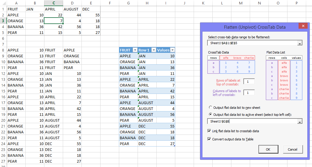
http://peltiertech.com/images/2015-02/DailyDoseUnpivotDataSMBDialog.png
It offers linking of the output to the original data, because you might decide that 7 oranges for April was 8, and it’s easier to find and replace in the crosstab table. Also it offers the option to turn the output range into a Table, because Tables are the bomb.
I’m working on an algorithm to autofill the entries for Rowes of Labels and Columns of Labels with something smarter than ones.
This is cool. Rarely does it take less than a day to build a whole new function for my utility.
The inputs and outputs in my comment were nicer, but WordPress turned the tabs into spaces, so they came out ugly. Click on the link to the image, and you’ll see it.
@Jon. Dick’s looked awfully long and convoluted. No Dick’s code doesn’t. Because it’s my awfully long and convoluted code, not his. :-)
My approach is actually several approaches in one, and a lot of its length is due to end cases that would otherwise not produce a PivotTable. I did a separate blog on it at http://dailydoseofexcel.com/archives/2013/11/19/unpivot-via-sql/ that discussed the approach. For instance, if unwinding a very large crosstab would result in a flat file that exceeds the amount of rows in Excel, it uses some dynamic SQL to create lots and lots of Union All statements, and then writes the result directly to a PivotTable. Otherwise it uses a second approach of straight out array manipulation. And it does a whole lot of checking around number formats and some other things that would otherwise cause an error in some circumstances. So it’s long, but it’s robust to quite a few things that your shorter code won’t handle.
Nice looking dialog, Jon. Shane Devenshire shared his Data Normalization Utility over at the DataProse blog some time back, which is worth a look see too. http://dataprose.org/2014/06/undaunted-by-unpivot-ii/
@Jon
You might have noticed that the structure of your table is quite different form the one Jeff used and on which my suggestion was based.
If you want to convert a matrix with rowlabels and columnlabels with the same appraoch you can use:
How would you modify unpiviot_smb so that it skips values with 0?
Jonathan: That’s a good requirement. One of the routines above has an option to skip blanks, but I never thought about also letting it skip zeros. I’ll rewrite the routine so that you can feed it an array of things to skip. Watch this space…
Hello Jeff,
Hoping you will pick up on this comment from your 2013 post! Thanks for the fantastic post, I’m utilizing your code for the “Multiple Consolidation Trick approach” and it’s working great. I was wondering if you’ll be willing to share a version of your code that is able to handle multiple header ROWS as well as columns? Something like this:
Country Sector 1990 1990 … 2009
Jan Feb … Jan
==============================================
Australia Energy 290,872 296,887 … 417,355
New Zealand Energy 23,915 25,738 … 31,361
United States Energy 5,254,607 5,357,253 … 5,751,106
Australia Manufacturing 35,648 35,207 … 44,514
New Zealand Manufacturing 4,389 4,845 … 4,907
United States Manufacturing 852,424 837,828 … 735,902
Australia Transport 62,121 61,504 … 83,645
New Zealand Transport 8,679 8,696 … 13,783
United States Transport 1,484,909 1,447,234 … 1,722,501
Into this:
‘ Country Sector Year1 Year2 Value
‘ ====================================================
‘ Australia Energy 1990 Jan 290,872
‘ New Zealand Energy 1990 Jan 23,915
‘ United States Energy 1990 Jan 5,254,607
‘ Australia Manufacturing 1990 Jan 35,648
….
‘ Australia Energy 1990 Feb 296,887
‘ New Zealand Energy 1990 Feb 25,738
‘ United States Energy 1990 Feb 5,357,253
‘ Australia Manufacturing 1990 Feb 35,207
….
I know it shouldn’t be too hard because it’s just doing the same “consolidate then split using text-to-column” approach that you did for the column headers, but I’m not very proficient with VBA so figured I should ask the guru(s).
Hi William. These days PowerQuery (built in to Excel 2016 and later and available as a free addin for 2010 or 2013) is the best tool for that particular job. Google PowerQuery and unpivot multiple columns and you should turn up heaps of tutorials. Look out for anything from Ken Puls on this subject. In fact, buy his book and consider his training…you won’t find a better guide!