It seems I have server-issue reprieve, so I’ll take advantage of it by throwing up the first post in weeks. Don’t worry, it’s not Excel related. I mean, who can expect that from this site. I do have a couple posts in the hopper, I just can’t seem to login when I want to write the up.

I got an email from an old friend asking for my recommendations for a new desktop computer. I wrote a longer reply than I expected and figured I might as well post it here. That way you can give your two cents in the comments. First, I’ll summarize his question/requirements:

I want “serious scientific/number-crunching/math-oriented”, and things labeled “home”, “office”, and “gaming” don’t seem like the right fit. I would like to use this machine primarily for compiled Python, S Plus, Mathematica, and C++ dll’s I am coding for Excel and OpenOffice. Specific points:

1. Is 8 GB RAM enough? Speed-wise, will 16 or more make a “significant” difference?
2. Which processor: i7?
3. Will a hybrid drive make any difference? Incidentally, I keep all of my documents on my NAS; I would, of course, keep development versions on the local HD, but really don’t need more than 150 MB (if that!) on it.
4. Dell looks good – highly configurable — what’s your take?
5. Monitor/Video Card: One of my Macs is 27″, and is awesome for my wife’s photo/cine avocation. I am writing you from a 17″ Mac ProBook. Works for me. So I won’t need a particularly large monitor (which one?!?); what I should do re the video card?
6. I/O: Several USB 3.0; Wired Ethernet, of course; Bluetooth; Thunderbolt. DVD and SD drives would be great.

Here’s my reply:

I don’t profess to be an expert, but I’m happy to give you my opinion. Just take it for what it’s worth. My last three desktops were 1) custom built 2) HP HPE-150f and 3) custom built.

My Last Three Computers

1. I read codinghorror.com about how he built his own home theater PC. I was cutting cable and needed something to run Windows Media Center for over the air TV. I somewhat followed his lead, but since mine would be out of sight, I didn’t worry about making it small or quiet. I wouldn’t recommend my particular build for your purposes because it was built with the new (at the time) Intel chipset that had HDMI out built-in.

   I was in a situation where I didn’t trust Dell anymore, didn’t know who to trust, and was interested in trying my hand at building hardware just for the experience. I made some errors along the way, but all-in-all it has been an outstanding machine. My biggest mistake was not buying a big enough power supply. I also had a hard drive go bad in the first year. Even with the missteps, the whole cost was about $1,400.

2. I was ready to replace my Dell desktop because it was 7 years old. I had a reasonably good experience building a PC so I was going to go that route again. It was a different build, so I there was still some chances to make mistakes, but I priced it out on New Egg anyway. Then I went to HP to see what a comparable machine would cost. It was a few hundred dollars cheaper and it didn’t really make sense for me to build it myself. I got an i7 2.8Ghz with 8 GB.

   That was four years ago, or so, and this machine has been terrific. Zero problems and it does everything I want performance wise. My only problem with HP is that they have a lot of craziness going on – they announced they were getting out of the PC business, then retracted. It just gives me pause. We use HP exclusively at work (~1,000 desktops) and they are probably still my go-to manufacturer.

3. The third desktop was for my son. It was still a better deal not to build it, but I wanted to give him the experience of building a PC from srcatch, so we went that route. It was a pretty good experience and it has been a good machine. If you’re interested in building your own, I’ll send you the component list.

Operating Systems

I run Win7 and my son runs Win8. He prefers Win8, but kids are stupid, so what are you going to do. On my HTPC, if I upgrade to Win8 I have to pay extra for Windows Media Center. In other words, I’m never upgrading. And when Win7 doesn’t work anymore, I’m going Linux/XMBC for the HTPC. Sorry Microsoft, but when you stopped building problems for guys like me you should have expected this.

Your Specific Questions

1. I bought my HP with 4 GB (the stock amount) and bought another 4 from crucial.com. You can save some pretty good money that way, but price it both ways. Just make sure you get enough slots if you’re going to add after market RAM. If I were buying today, I wouldn’t get less than 12 GB because RAM is so cheap that even an incremental increase in performance is worth it. I’d look at 16 too. But really, I’ve been running 8 GB for a while, and I have no problems, so it might be a waste of money.
2. I like my PCs to last 5-7 years, so I tend to over buy on CPU and RAM. I don’t what’s newer and better than i7, but I definitely would not go with i5.
3. Another misstep on building my own was not having an SSD for a boot drive. If I were building again, I would get an SSD for a primary and a Western Digital for storage. SSDs are getting more reliable at a pretty quick pace.
4. Six years ago, or so, I stopped buying Dell. I bought them exclusively for home and work for the 10 years prior, but the quality of the components was going down and I’d had enough. I’ve heard they’ve made a bit of a comeback, quality wise, but I’m not sold yet. Concurrent with them buying cheaper parts, they moved their customer service to India. Back in the day when I didn’t have to talk to Dell customer service because their shit just worked, I wouldn’t care where it was. But with failing parts, it was a problem. I’m not trying to denigrate an entire sub-continent. It was just that the company Dell hired really sucked. I’m sure the rest of India is very knowledgeable.
5. I have two 22″ monitors side-by-side and love it. I can’t imagine coding in Excel without the VBE on one screen and Excel on the other. Even when I code in Ruby, Python, Java or whatever, I need to have stackoverflow on one screen and the IDE on the other. I will never have one monitor again – it is the single best productivity boost in my computing career (including my keyboard shortcut mania). Both my monitors are Acer that I got from Newegg. They’re slightly different heights, but I find that piano sheet music books level them up nicely. If you can get identical, that’s even better. My work monitors are identical 22″ ASUS and I’m very happy with those too.
6. Don’t sacrifice on USB ports. They don’t all have to be 3.0, but make sure you have double what you think you need. Even if you don’t go with two monitors, you should consider a dual output video card in case you change your mind.

I’m a couple years away from replacing my desktop, but if I were forced to do it, I would price out HP, Lenovo, and Asus. And probably Dell for good measure, but I would have to be really convinced to go back to Dell. Lenovo and Asus have awesome reputations in laptops and I don’t know why that wouldn’t translate to desktops. I bought a used Asus convertible tablet several years ago and it still runs like a champ.

End of reply

If you have any opinions on desktop hardware, please leave them in the comments.

Hey, did you notice that this page loaded in a few milliseconds instead of timing out? Me too!

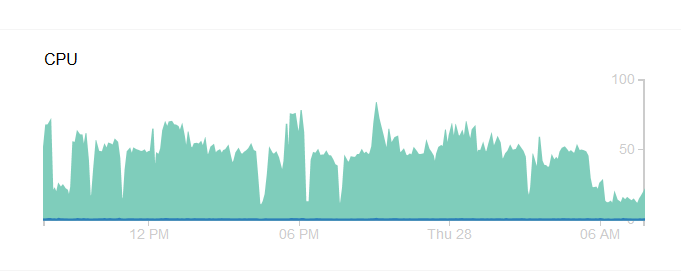
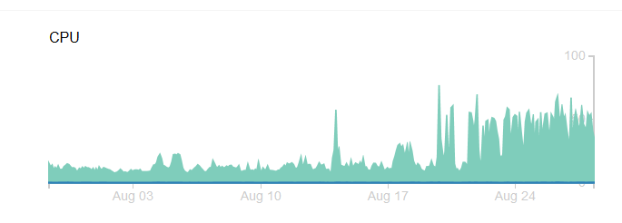
I don’t know what caused that period of slow down because I don’t know much about servers. I know my CPU percentage has been higher lately. Here’s what it looks like over the last 30 days.

And over the last 24 hours.

Last night I created a support ticket with Digital Ocean. And today it miraculously works. It makes me suspicious, but I can’t imagine a business model where you throttle your customers until they call you on it. I mean except for the cable and cell phone industries.

So I’m going to enjoy it while it lasts. I’m also going to get in an Excel post today before I have more problems.

Over at the Excel Guru forum, Yewee asks:

I have 3 sheets in my excel worksheet.

1. Org
2. DataSource
3. Pivots Table

My Pivot table will get the data from the DataSource sheet. I will like to have the filter of the Pivot Table from one of the cell in Org Sheet.

How can I do that?

Incredibly easily, if you have Excel 2010 or later…because:

• a PivotTable with nothing but one field in the Filters pane looks and behaves pretty much exactly like a Data Validation dropdown does; and
• that PivotTable can be hooked up to the other PivotTables via slicers, so that it controls them.

If you’re a long-time reader of this blog you probably already know that, and may want to skip to the end to find a bit of VBA that makes setting up Slicers slightly more easy. But if you came here via Google, then pull up a pew and read on.

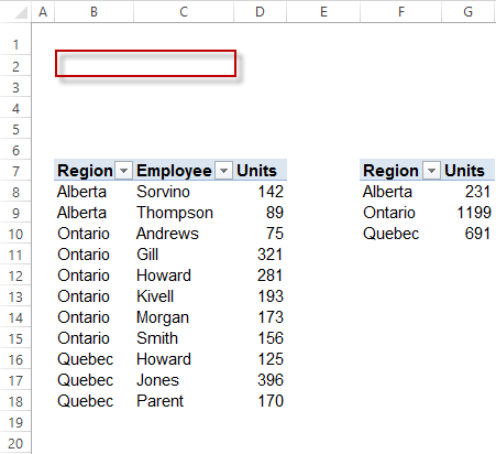
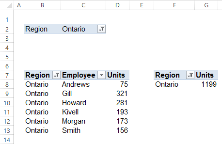
So let’s say these are the two Pivots that you want to control via a dropdown, and you want to put the dropdown where the red rectangle is:

 
 

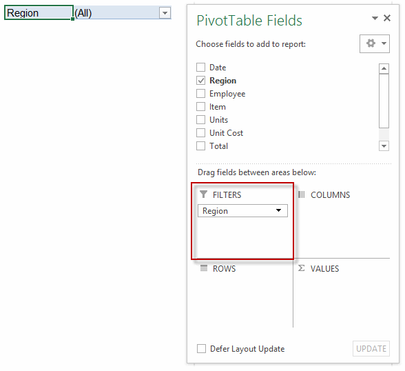
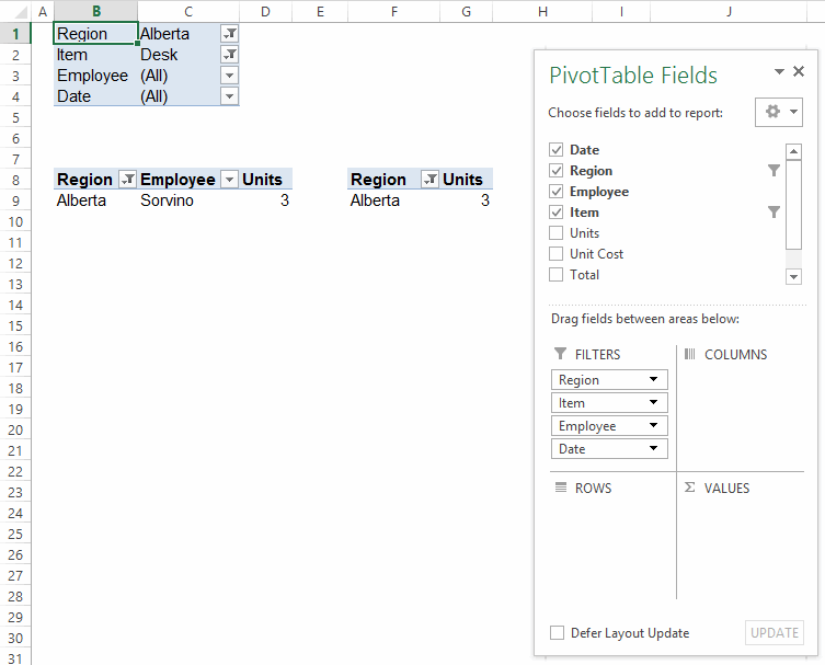
First, create a new PivotTable from the datasource that the other pivots share (or make a copy of one of the existing Pivots) and in the PivotTable Fields pane add the field you want to filter the other Pivots by to the Filters pane. (If you created this Pivot by copying another, remove any other fields that might appear).

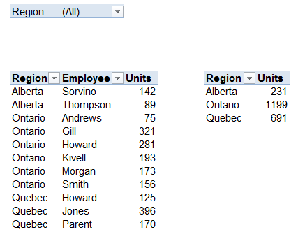
Great: Now you have a PivotTable masquerading as a Data Validation Dropdown. From now on, I’ll call it the ‘Master Pivot’. So just drag that Master Pivot where you want it:

 
 

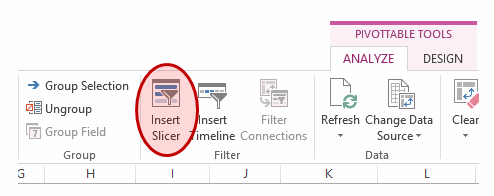
From the ANALYZE tab of the PivotTable Tools contextual menu in the ribbon, click the Insert Slicer icon:

 
 

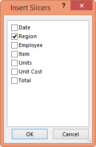
…and from the menu that comes up, choose the field name that matches the field you put in the Master Pivot:

 
 
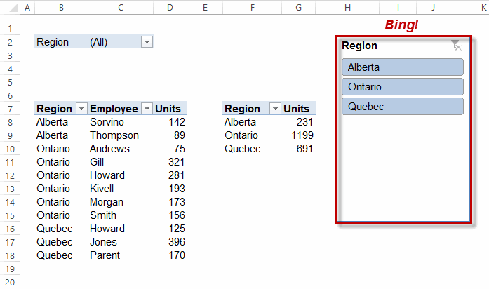
…and your slicer will magically appear:

 
 

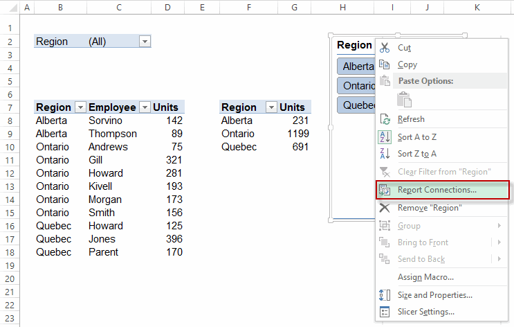
Now we connect that Slicer to the other PivotTables. To do that, right click on the Slicer that just appeared, and click the Report Connections option:

 
 

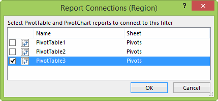
You’ll see from the Report Connections box that comes up that currently it’s only connected to one PivotTable – which of course is the Master PivotTable that we used to insert the slicer in the first place:

 
 

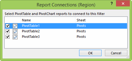
What we want to do is connect it to the other PivotTables, by checking those other checkboxes:

 
 

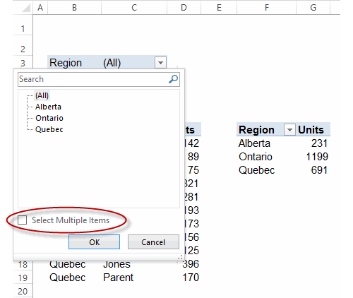
(Optional) We might want to make it so that the user can only select one thing at a time by clicking on the Master Pivot filter dropdown, and unchecking Select Multiple Items, if that’s your intent:

 
 

…and now all we need to do is move that Slicer somewhere out of sight (but don’t delete it):

 
 

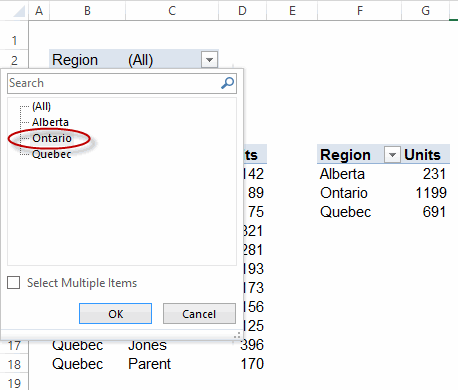
Now when we select a region from that Master Pivot dropdown…

 
 
… all the other Pivots are filtered to match:

 
 

That’s it…job done. As simple as possible, and no simpler.

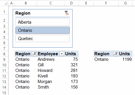
Actually that’s a lie…unless there’s a good reason not to, it’s much simpler just to use a Slicer in the first place, and not bother with setting up the Master Pivot dropdown at all:

 
 

Of course, that Slicer takes up much more room than our Master Pivot dropdown. So maybe that’s a good reason to use the Master Pivot approach, and not a slicer. Especially if we might want more than one dropdown to control all the Pivots and space is at a premium:

Or you can do away with the Master Pivot altogether, and just set the slicers up between the actual ‘output’ pivots themselves, so that as soon as they change a PivotFilter setting in one of the Pivots, the others get changed too. (Note that this also happens with the ‘Master Pivot’ approach…it’s just that we don’t actually need to have that Master Pivot sitting there taking up space at all).

Programatically add and connect Slicers

I’ve always found it annoying that there’s no right-click option to add a Slicer to the currently selected PivotField. Plus connecting Slicers to multiple PivotTables is a drag. And also, I hate it how it adds new Slicers over the top of old slicers. So here’s some code that remedies all that:


Sub AddSlicer()
Dim pt As PivotTable
Dim ptOther As PivotTable
Dim pf As PivotField
Dim pc As PivotCache
Dim rng As Range
Dim sc As SlicerCache
Dim varAnswer As Variant
Dim bFoundCache As Boolean
Dim rngDest As Range

Set rng = ActiveCell

On Error Resume Next 'in case user has not selected a PivotField
Set pt = rng.PivotTable
Set pc = pt.PivotCache
Set pf = rng.PivotField
On Error GoTo 0

If pt Is Nothing Then Exit Sub

If pf.Orientation <> xlDataField Then
Set rngDest = Intersect(ActiveCell.EntireRow, ActiveCell.Offset(, ActiveCell.CurrentRegion.Columns.Count + 1))
On Error Resume Next 'SlicerCache might already exist
With rng
If pt.PivotCache.OLAP Then
Set sc = ActiveWorkbook.SlicerCaches.Add2(pt, .PivotField.CubeField.Name)
Else: Set sc = ActiveWorkbook.SlicerCaches.Add2(pt, .PivotField.Name)
End If
sc.Slicers.Add SlicerDestination:=ActiveSheet, Top:=rngDest.Top, Left:=rngDest.Left
End With
If Err.Number > 0 Then 'SlicerCache already existed. Work out what it's index is
On Error GoTo 0
For Each sc In ActiveWorkbook.SlicerCaches
For Each ptOther In sc.PivotTables
If ptOther = pt Then
bFoundCache = True
Exit For
End If
Next ptOther
If bFoundCache Then Exit For
Next sc
End If

varAnswer = MsgBox(Prompt:="Make Slicer control the " & pf.Name & " field in all Pivots on the same sheet?", Buttons:=vbYesNo)
If varAnswer = vbYes Then
For Each ptOther In ActiveSheet.PivotTables
If ptOther.CacheIndex = pt.CacheIndex And ptOther.Parent.Name = pt.Parent.Name Then
sc.PivotTables.AddPivotTable ptOther
End If
Next
End If

Else: MsgBox "You can't add a Slicer to a Values field."
End If
End Sub


In addition, the below code will add the Add Slicer icon to the right-click menu that comes up when you right click on a PivotField:

Option Explicit

Private Sub Workbook_Open()
AddShortcuts
End Sub

Private Sub Workbook_BeforeClose(Cancel As Boolean)
DeleteShortcuts
End Sub

Sub AddShortcuts()
Dim cbr As CommandBar

DeleteShortcuts

Set cbr = Application.CommandBars("PivotTable Context Menu")

With cbr.Controls.Add(Type:=msoControlButton, Temporary:=True)
.Caption = "Add Slicer"
.Tag = "AddSlicer"
.OnAction = "AddSlicer"
.Style = msoButtonIconAndCaption
.Picture = Application.CommandBars.GetImageMso("SlicerInsert", 16, 16)
End With

End Sub

Sub DeleteShortcuts()

Dim cbr As CommandBar
Dim ctrl As CommandBarControl

Set cbr = Application.CommandBars("PivotTable Context Menu")

For Each ctrl In cbr.Controls
Select Case ctrl.Tag
Case "AddSlicer"
ctrl.Delete
End Select
Next ctrl

End Sub


…meaning whenever I right click on a PivotField I get this:

 
 

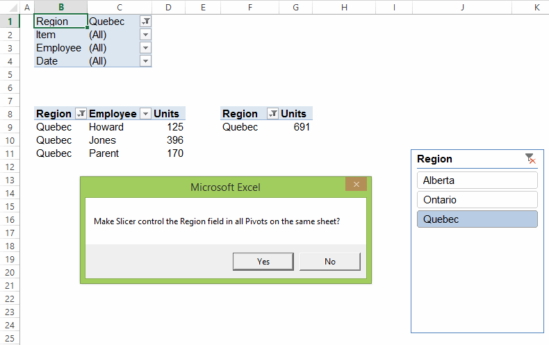
Clicking on that adds a Slicer to the selected field automatically, plus asks you:

 
 

Hell yes, I do!

Here’s a sample file:
Sync-PivotTables-from-dropdown_20140818

 
 

Found a couple of funny bugs today that I thought I’d share.

First, this one:
 

 

Weird: Partially italicizing right-aligned text screws with the display of trailing spaces. But it doesn’t do the same to left-aligned text with leading spaces:
 

 

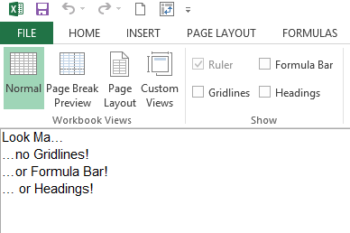
And then there’s this one, where you start with a file that you’ve suppressed gridlines on:
 

 
…and then you add a New Window…which allows you to look at a different parts of the same file on dual monitors – or even the same monitor if it’s suitably wide, by clicking on this:
 

 

(Aside: I never rated this feature as being particularly useful until I got a second monitor and then recently rediscovered it. Now I’m starting to think is indispensable, as I no longer have to scroll around half as much as I do when getting to grips with how spreadsheets are laid out, or when putting in new formulas that point from one region of a workbook to a completely different region of the same workbook. I’m sure Dick has been using it for years to avoid rodenting.)
 

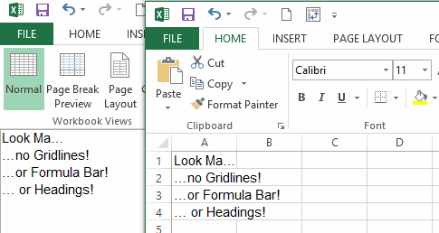
But when you compare the new window (which Excel temporarily renamed SomeFileName:2) to the old (which Excel temporarily renamed SomeFileName:1), there’s a couple of subtle differences:
&nbps;

 

So it respects my wishes to not show the Formula bar, but ignores my wish to not display gridlines and headings. And if I close the original window – the one called SomeFileName:1 – then those settings I didn’t want from SomeFileName:2 are now in the file SomeFileName. Bummer.

So make sure that’s the one you close when you’re done. Otherwise your file now has gridlines and/or headings when you didn’t want it to.

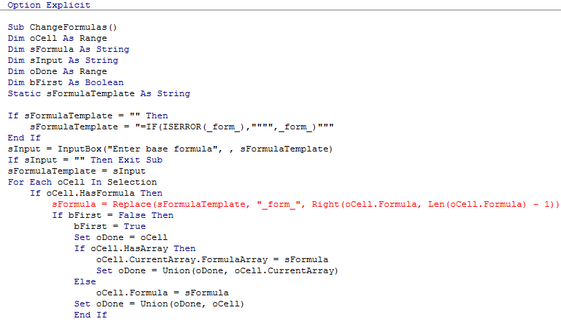
Sometimes when I copy code from the web and paste it into VBA, I get something like this:
 

 

…and I’m damned if I know why. It’s not the usual culprit of incorrect quote marks. It’ something else, and I don’t know what.

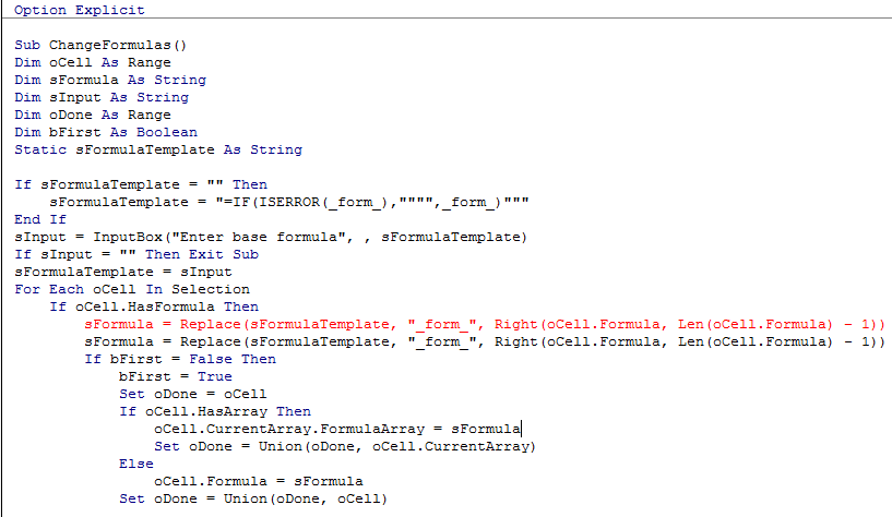
Usually I just retype the offending line:
 

 
…and after looking in vain for a difference, simply delete the bad one, and put it down to inexperience.

But not today. Because I’m tired of being compiled around. So today, I’m gonna find out why. And I’m going to use Excel to keep VBE honest. Conquer and #DIV/0, I say.

If I paste the two formulas into separate cells in Excel, then I can clearly see that something is amiss. I just can’t clearly see the actual something:
 

 

Okay, let’s get nasty, and atomise these suckers so I can compare their DNA:
=MID(A,ROW(A1:INDEX(A:A,LEN(A))),1)
=MID(B,ROW(B1:INDEX(B:B,LEN(A))),1)

 

Well take a look at that…there’s the culprit:
 

 
No wonder I couldn’t see it:
 

In this particular case, the culprit looks like Ken Pul’s Blog platform…I stole the code from a comment Jan Karel left there, and note that the code has no similar issue if I lift it directly from Jan Karel’s site.

There you go. Busted.

Makes me feel like singing:

Behind the scenes, Excel does quite a bit of smart rationalisation in terms of SlicerCaches whenever you connect Slicers to mulitple PivotFields, and this can be a bit confusing if you’re not familiar with what’s going on. So let’s take a look-see.

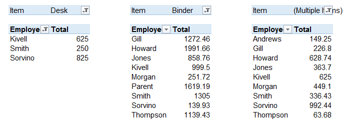
First, let’s create three PivotTables all based on the same data source – meaning they all share the same PivotCache and therefore can all be connected – or ‘daisy-chained’ – together with Slicers later on if we so desire:
 

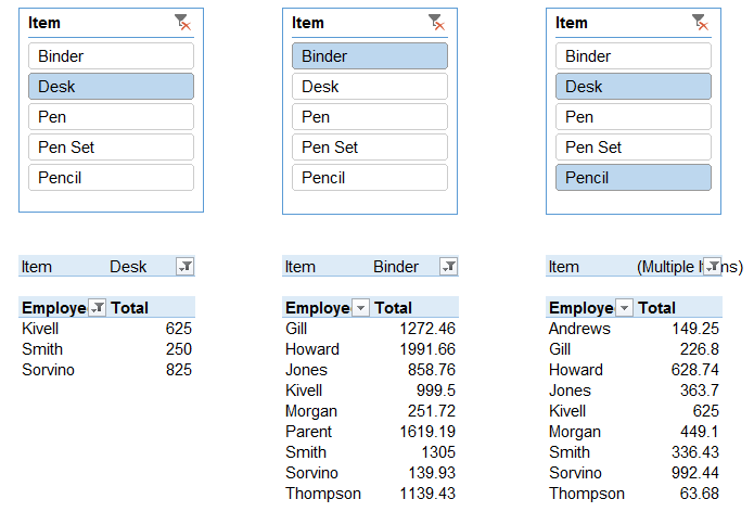
Next, let’s add a separate Slicer for each of them, with each Slicer pointed at the “Item” field of it’s related Pivot:
 

 
 
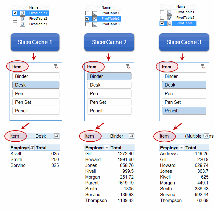
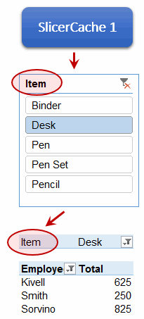
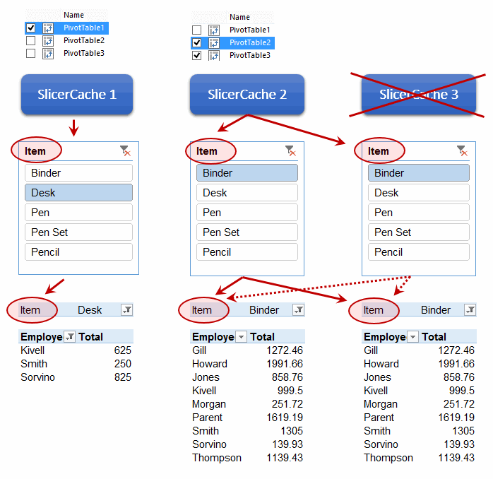
So that’s what we see. How does Excel see this?

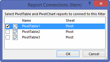
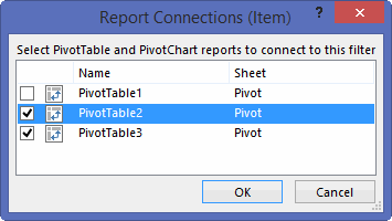
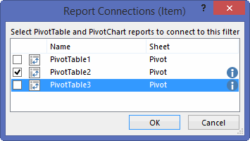
There’s a couple of points to note about this diagram. Firstly, the boxes across the top are screenshots from the Report Connections dialog box:
 

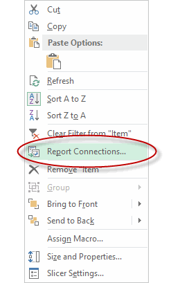
…which you get by right-clicking on a Slicer and selecting this:
 
< And secondly, the reason I've drawn circles around those Item fields:  

…is that I really want to underscore that slicers operate at the PivotField level, not on PivotTable level.
 
So where where we. Ah yes, three Pivots based on the same PivotCache, with three Slicers all pointing at the Item field of their respective PivotTable:
 

Let’s now change Slicer Two so that it also points at the Item field of PivotTable Three:
 

 
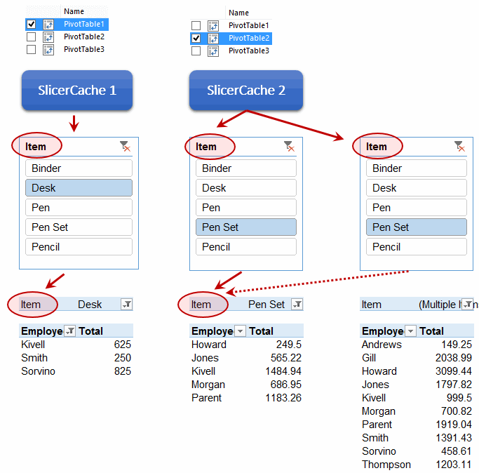
How did that change the conceptual lay of the land?

 
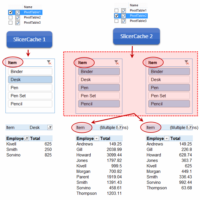
Well, that looks different. Excel rationalised the SlicerCaches by ditching SlicerCache three, and now both Slicer Two and Slicer Three are connected to SlicerCache Two. Meaning that conceptually, they both point at the Item field in both PivotTable2 and PivotTable3. In fact, if you were to right click Slicer Three and look at the ReportConnecitons, you’d see it looks exactly the same as for Slicer 2, even though we didn’t touch it. And if we change the selection in one of these Slicers, we see it replicated in the other as well as in each Pivot. It’s as if those Slicers are one and the same:

 
Interestingly, if we remove PivotTable3 from that SlicerConnections dialog:
 

 
…things don’t go back to the way before: Slicers Two and Three are still synced together, but control PivotTable2 only. PivotTable3 is completely slicer-less:
 

There’s no way you can get that Slicer Three to operate independently on its own again. You’ll just have to delete it and add another, I’m afraid.

Adding Slicers Programatically

 
If you record a macro while adding a slicer, you get code like this:

ActiveWorkbook.SlicerCaches.Add(ActiveSheet.PivotTables(“PivotTable1”), “SomePivotField”). _
Slicers.Add ActiveSheet, , “SomePivotField”, “SomePivotField”, 146.25, 309.75, 144, 187.5


All those arguments of the Slicers.Add command are optional except the first. And all those numbers just tell Excel where you want the Slicer, and how big you want it to be. So you could just go ahead and use this for the same result:

ActiveWorkbook.SlicerCaches.Add(ActiveSheet.PivotTables(“PivotTable1”), “SomePivotField”). _
Slicers.Add ActiveSheet


You can actually add a SlicerCache that controls a pivot without adding a Slicer:
ActiveWorkbook.SlicerCaches.Add ActiveSheet.PivotTables("PivotTable1"), "SomePivotField"

…and then you can connect another PivotTable to it:
ActiveWorkbook.SlicerCaches("Slicer_SomePivotField").PivotTables.AddPivotTable (ActiveSheet _
.PivotTables("PivotTable2"))

…meaning you now have an invisible slicer that keeps the pivots in sync, based on user selections from the pivot filters themselves. Spooky! Note that –

• If you add another slicer to that same PivotField on either of those PivotTables, Excel simply uses the slicer cache you just set up, meaning the new slicer controls BOTH pivots, even though you just added it to one.
• If you delete that slicer, Excel performs a Slicer Exorcism: it deletes the underlying SlicerCache, meaning your two pivots are no longer synced. Unspooky!

Here’s something else slightly spooky. Or rather, kooky. Normally if you delete a pivot that is the ONLY pivot that uses a particular PivotCache, Excel gets rid of the PivotCache automatically. Excel basically thinks “Well, we won’t need that crap lying around anymore”. But strangely, if you have a slicer set up for that pivot, then deleting the pivot leaves both the slicer AND the pivot cache alone. The PivotCache only gets deleted once you delete that orphaned slicer.

Well, that’s enough for today. But *HORROR* there’s some Slicer-related sequels coming to a screen near you soon:
 

So stay tuned. And awake.

Welcome back to Twice Daily Dose of Excel. Heck, these days we’re more regular than Julian Assange’s visits to the Ecuadorian Embassy!

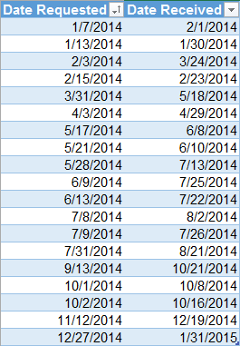
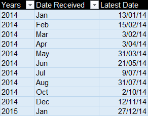
Audrey has a table that looks something like this (if you’re American):

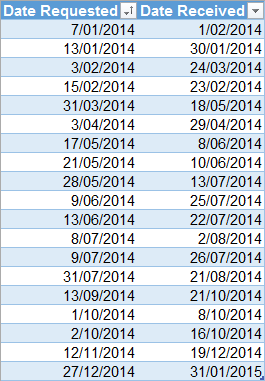
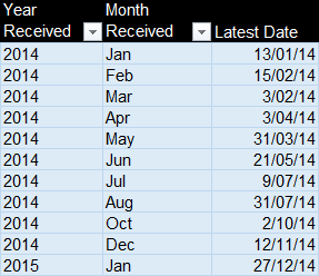
…or like this (if you live somewhere sensible, like in New Zealand and a good deal many other places besides):

She uses this to track when she requested a piece of information from someone, and the date she received a response. I’m picking she’s NSA, and is asking Julian – who is actually a quadruple agent – whether he needs more sun lamps. Stranger things have happened, recently.

Anyways, she’d like a formula to find the oldest/latest request date out of all responses received in a particular month.

She could array enter something like this, which will do the job without any need for helper columns:

=MAX($A$2:$A$20*(DATE(YEAR($B$2:$B$20),MONTH($B$2:$B$20),1)=DATE(YEAR($B2),MONTH($B2),1)))

…which to an Excel Pro with a lifetime of formulas under their belt would look like this:

=NOT(RocketScience)

…but to anyone else:
="Αυτό θα μπορούσε κάλλιστα να είναι γραμμένο στην ελληνική γλώσσα"

You could debate whether there’s a right formula to use in a situation like this. In fact there’s some great debate on that original blogpost as to whether one proposed solution is awesome, potentially obfuscating, or incomprehensibly mutant. So with this in mind, is there a right formula to use in this case? Depends on who’s trying to comprehend what’s happening here in 6 months time. Perhaps yourself, with six more months of grey-matter dieback under your belt. Or hat, rather. Is there a right non-formula approach to Audrey’s problem? You betcha:

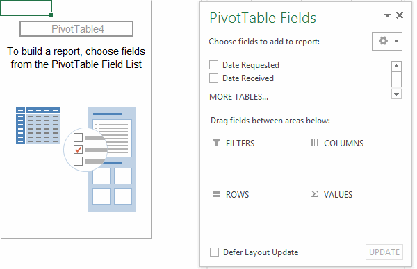
Just create a PivotTable out of that sucker:

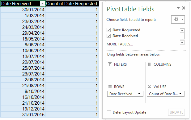
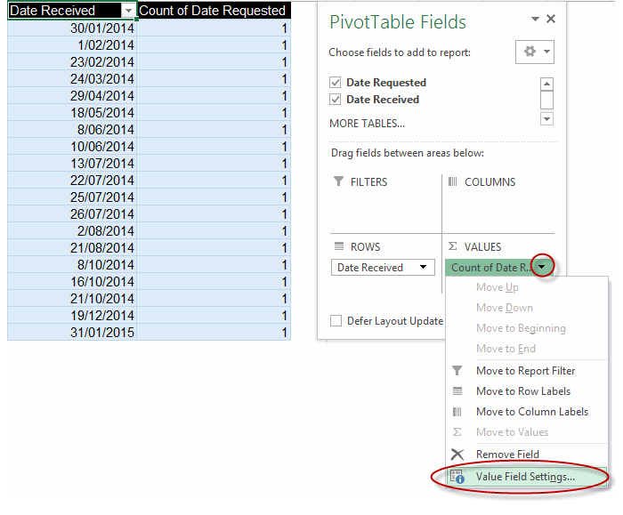
…drag the ‘Date Received’ field to the Rows pane and the ‘Date Requested’ field to the Values pane:

…launch the Value Field Settings dialog for the Date Requested field:

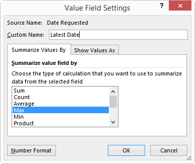
…change the name of the Date Received field to something meaningful, and change Sum to Max:

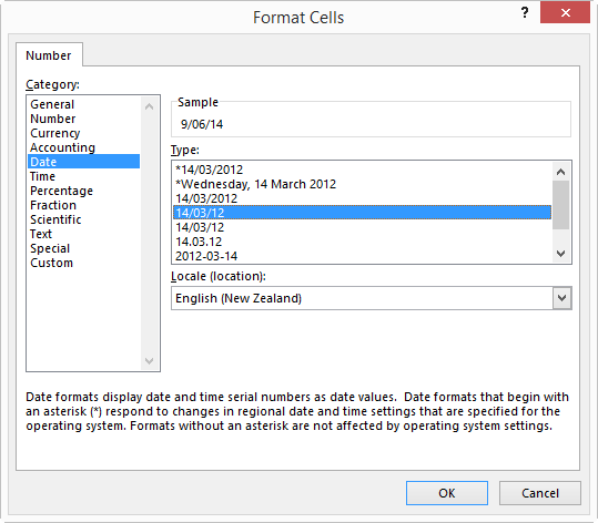
…plus click on that Number Format button while you’re there so you can change the format to Date:

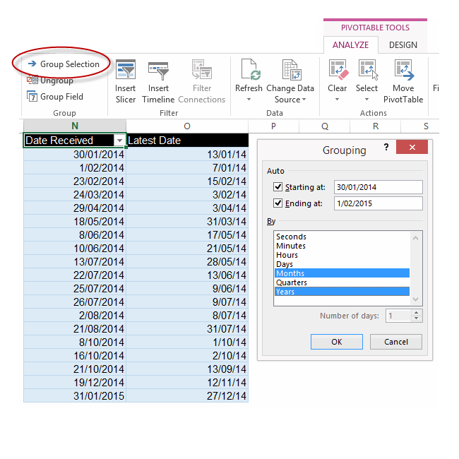
…then select any cell in the Date Received column and click Group Selection from the PivotTable Tools > Analyze contextual tab, and group by Months and Years:

…and exhale:

No, wait…hold that breath…we forgot to change the name of that ‘Years’ column that just appeared – as well as the ‘Date Received’ column that now holds Months only – to something more suitable:

Now exhale.

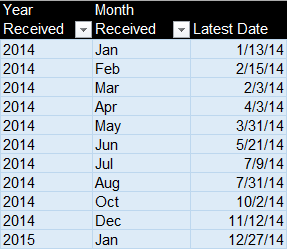
Here’s the genius…it even works in American:

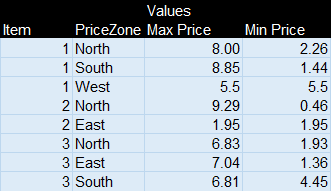
…and it works on trickier problems, like the original one at that post:

 
¿Fórmulas? No nos hacen falta fórmulas apestosas!

GMF comments:

I use XY charts for schedules and I like to have a vertical line showing today’s date. I do this so frequently I have a named range for each of the X and Y values. To get the current date to show up as 2 similar X values the best I could come up with is:

=(ROW(INDIRECT(“1:2″))/ROW(INDIRECT(“1:2″)))*TODAY()

There must be a better way, but I can’t just put ={TODAY(),TODAY()} as a value and I’m curious why.

Until somebody smart like Charles Williams jumps in with a better explanation, the reason you can’t put individual functions into an array is that you can’t. I know, it sucks. I’d like to be able to do that too.

Edit: Colin Legg beat Charles to it:

When you use { } within a formula they are delimiters for an array constant. The formula parser won’t let you embed functions or references within an array constant because, by definition, the elements wouldn’t be constant anymore.

That said, you can get there indirectly:
=TODAY()*{1,1}
={41854,41854}

Sure Jeff, but I want to be able to put different functions in each array position.

Not a problem…with a bit of cleverness, you can do the equivalent of this:
={MIN(SomeRange),Max(SomeRange)}

…like this:
=MIN(SomeRange)*{1,0}+MAX(SomeRange)*{0,1}

…which says to Excel:

• Populate a 2-element array with the minimum of SomeRange, but multilpy the first element by 1 and the second element by 0, in order to clear the minimum from that second element.
• Populate a 2-element array with the maximum of SomeRange, but multilpy the first element by 0 and the second element by 1, in order to clear the maximum from that first element.
• Add them together, leaving just the minimum in the first, and the maximum in the second.

 
 

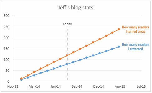
So how does this tie in with what GMF wants to do, i.e. put a vertical line in an XY chart to show the current date?
 

Well, because this is an XY chart, you only need two coordinates to draw that date line line: the point at the bottom, and the point at the top.

So to get the X values we want – today’s date, we define a name called Today:
=TODAY()*{1,1}
And for the Y values – the Min and Max values across both ‘Values’ series – we define a name called MinMax:
=MIN(SomeRange)*{1,0}+MAX(SomeRange)*{0,1}

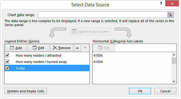
And then we can add a new series called Today to our chart:
 

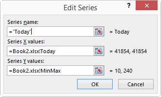
…with the X and Y coordinates of that series pointing at the appropriate name:
 

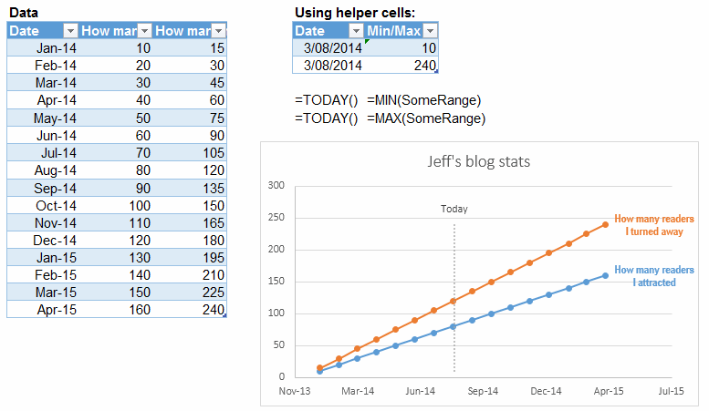
Of course, you don’t actually need a Named Range to do this… you can simply have some helper cells in the actual worksheet that calculate the Min and Max values of the entire block of data, and point your Today series at that:
 

Here’s a sample file with both approaches: Todays Date on ScatterPlot

Maybe this stuff is all included in Dick and Mike’s book 101 Ready-To-Use Excel Formulas. I don’t know…I’m still waiting for my free advance copy in the post.

Well, that’s all folks. Hopefully this post moved those lines on the chart closer together rather than pushing them apart.