Hey Dick, thanks for having me over. Wow, it’s even nicer in here than I imagined. Look at all those posts! Hey, is that an Office XP beer stein… where’d you get that? Gosh, do you really wear all these baseball caps?
Okay, well great to be here. I hope I don’t blow it. I’m going to talk about a fairly pedestrian topic, but one I deal with daily as a data analyst and report writer: comparing versions of output data.
At my work we have a report modification and publication process to verify that they’re outputting reasonable results. A lot of times this means comparing a report to its previous published version and confirming that the outputs are identical before moving on with the process.
I’ll show some tricks I use to do these comparisons. Please note these examples all assume the data you’re comparing is easily re-creatable, e.g., it comes from a data connection or was exported from another tool. In other words, don’t do these tests on the only copy of your output!
The Most Basic of Tricks – Comparing Sums
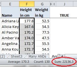
One quick trick you’ve probably used is to grab an entire column of output and check its SUM in the status bar. Aside from comparing row counts, this is about as simple as it gets.
I usually just look at the first three or so digits and the last three or so, mumble them to myself, switch to the other column and mumble those to myself. If my mumblings match, I call it good.
Mind you, I only do this as an informal check. Still, writing this got me to wondering how reliable it is, and about the likelihood of a false positive, a coincidental match. So I did a little test and filled two columns with RandBetween formulas then wrote a bit of VBA to recalculate them repeatedly and record the number of times their sums matched. With two columns of 1000 numbers, each filled with whole numbers between 1 and 1000, I averaged around three matches per 100,000 runs, or a .003% chance of a coincidental match. That’s a pretty small range of numbers though, equivalent to a span from one cent to ten dollars. So I upped it to whole numbers between one and a million, similar to one cent to 10,000 dollars. With a million calculations of 1000 rows there were no coincidental matching totals.
A More Thorough Trick – Compare All Cells
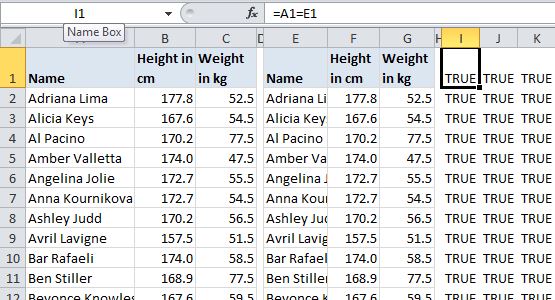
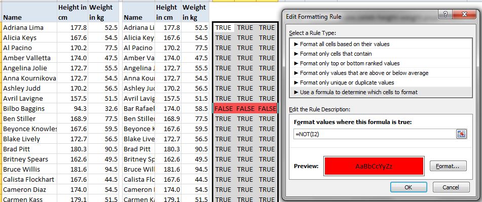
When I really want to make sure two sets of data with the same number of rows and columns match cell for cell, I do the obvious and … compare every cell. That could look something like this (but eventually won’t, so stick with me):
The two sets of data (a modified version of the indispensable table from celeb-height-weight.psyphil.com) are on the left, with the comparison formulas for each cell on the right. In this case they all match and return TRUE:
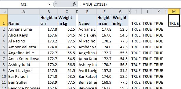
If you’ve got more than a few columns and rows, you probably don’t want to scan all the comparison cells for FALSEs. Instead, you can wrap up all these comparisons in a single AND, like this. It will return FALSE if any of the referenced cells are FALSE:
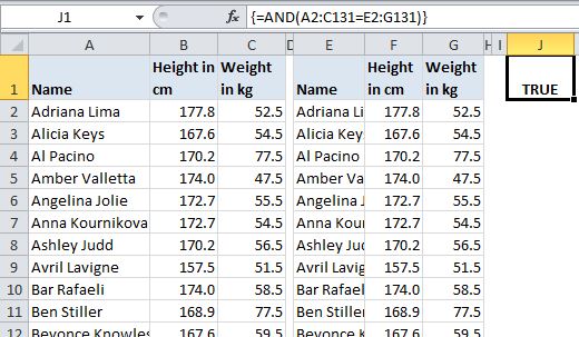
Or just eliminate the middleperson altogether with a single AND in an array formula:
What If They Don’t All Match?
If they don’t all match you can add conditional formatting to highlight the FALSEs…
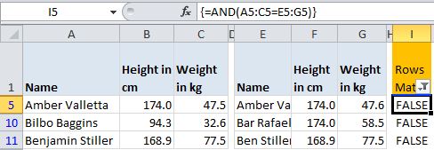
… or just add it directly to the two tables. However, rather than conditional formatting I’d use a per-row AND array formula and filter to FALSE:
Same Data, Different Order
Sometimes my rows of data are the same, but they’re out of order. I try not to yell at them like Al Pacino. Instead I might test them with a COUNTIF(S) formula, like so, which just counts how many times the name in a the second table appears in the first table:
=COUNTIF($A$2:$A$131,E2)
To compare whole rows, you’re stuck (I think) with longer COUNTIFS formulas than I care to deal with. I’d rather concatenate the rows and compare the results with a COUNTIF. I don’t have many worksheet UDFs in my tools addin, but one exception is Rick Rothstein’s CONCAT function, which I found on Debra’s blog. It’s great because, unlike Excel’s Concatenate function, it allows you to specify a whole range, rather than listing each cell individually.
COUNTIFs can get slow though once you’ve got a few thousand rows of them. So, another approach is just to sort the outputs identically and then use an AND to compare them. Here’s a function I wrote to sort all the columns in a table:
Sub BlindlySortTable()

Dim lo As Excel.ListObject

Dim loCol As Excel.ListColumn
Set lo = ActiveCell.ListObject
With lo
.Sort.SortFields.Clear
For Each loCol In .ListColumns
.Sort.SortFields.Add _
Key:=loCol.DataBodyRange, SortOn:=xlSortOnValues, Order:=xlAscending, DataOption:=xlSortNormal
Next loCol
With .Sort
.Header = xlYes
.MatchCase = False
.Apply
End With
End With
End Sub
At this point I should mention that I almost always work with Tables (VBA ListObjects) when doing these comparisons. A lot of the time I’ve stuffed the SQL right into the Table’s data connection. If the data is imported from something like Crystal Reports, I’ll convert it to a table before working with it.
Using Pivot Tables For Comparing Data – Fun!
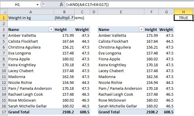
As I get farther along in a report’s development, odds are I might just want to compare a subset of the old version to the whole new version, or vice-versa. Using pivot tables is great for this. Say for instance my new report is only for people whose weight is under 48 kilograms. I’d like to compare the output of the new report to a filtered list from the older version and confirm that I’m returning the same weights for the people in the new subset. A pivot table makes this easy:
The pivot on the left, based on the original data, has been filtered by weight and compared to the pivot on the right, based on the new, less-than-48 data. An AND formula confirms whether the data in the new one matches the original.
I was doing this the other day with multiple subsets, causing the pivots to resize. I thought “wouldn’t it be cool to have a function that returns a range equal to a pivot table’s data area?” The answer was “yes,” so I wrote one. It returns either the used range or the data area of a table or pivot table associated with the cell passed to it. Here’s the code:
Public Enum GetRangeType

    UsedRange    '0

    'CurrentRegion - can't get to work in UDF in worksheet, just returns passed cell

    PivotTable    '1

    ListObject    '2

End Enum
Public Function GetRange(StartingPoint As Excel.Range, RangeType As GetRangeType) As Excel.Range
Dim GotRange As Excel.Range
With StartingPoint
Select Case RangeType
Case GetRangeType.UsedRange
Set GotRange = .Worksheet.UsedRange
Case GetRangeType.PivotTable
Set GotRange = .PivotTable.TableRange1
Case GetRangeType.ListObject
Set GotRange = .ListObject.Range
End Select
End With
Set GetRange = GotRange
End Function
The array-entered formula in H1 in the picture above becomes…
=GetRange(A3,1)= GetRange(E3,1)
… where 1 is a pivot table. You’ll note that the code itself uses the enum variable, which would be great if you could use the enums in a UDF. Also, you’ll see that I tried to have a cell’s CurrentRegion as an option but that doesn’t work. When returned to a UDF called from a worksheet, CurrentRegion just returns the cell the formula is in.
So Long
Okay then, see you later Dick. Thanks again for the invite. It means a lot to me.
No, no, don’t get up… I can show myself out and it looks like you’re working on something there. Wait a minute… no it couldn’t be… for a second there it looked like you were using a mouse… Must have been a trick of the light.
Cheers!
In a shopping basket the order of the Items do not matter.
So to compare two columns where Items are in different order you can use a single cell array formula
=AND(COUNTIF(List1,List2)*COUNTIF(List2,List1))
Returns a true/flase
Hi Doug. No, not a mouse. It’s a rat. I upgraded.
Funny you should mention PivotTable ranges. To me this is one of the most blindingly obvious oversights that MS has made in recent years. I can’t fathom why one of Excel’s oldest, coolest tools hasn’t been given some of the same chops an one of Excel’s newest, coolest tools (Tables). I’m feverishly writing a book on Excel efficiency, and spend a lot of time in it pimping PivotTables so that they do what they ought to right out of the box, and dynamic range functionality is right at the top. When it’s not so late and my rat’s not so tired I’ll give your code a lookover. But it’s time for us to both snuggle into bed.
Thanks Doug. You’re supposed to pimp your own site when you post here. I’ll do it for you. http://yoursumbuddy.com/blog/
For comparing line items, I like to use =–EXACT(CellOne,CellTwo), which converts TRUE/FALSE to 1 or 0. Doing this allows you to see the sum in the statusbar.
I’ve also taken inspiration from this post: http://dailydoseofexcel.com/archives/2014/02/10/subtracting-cells-in-the-status-bar/
to have the statusbar show how many unique items in are the selection, and if two columns are selected, show if they match.
That’s supposed to be to consecutive subtraction signs = – – EXACT(CellOne,CellTwo)
@Jeff, as Dick points out, this is a good time to flog my blog (yikes!) so here’s links to a few yoursumbuddy pivot-table-related posts. The first one specifically addresses the issue you raise:
A function to create dynamic named ranges for pivot table fields and data area. I know you’ve read it because your comment was longer than the post :-) http://yoursumbuddy.com/create-pivot-table-named-ranges/
A function to re-apply pivot table conditional formatting after a refresh obliterates it (a problem that cropped up starting in Excel 2007): http://yoursumbuddy.com/re-apply-excel-pivot-table-conditional-formatting/
My Unified Methodology of Pivot Table Formatting: http://yoursumbuddy.com/unified-method-of-pivot-table-formatting/
Sam: re your comment In a shopping basket the order of the Items do not matter.
That’s what my wife thinks. No matter how many times I politely inform her otherwise, she always puts the bread and eggs at the bottom, and the beer at the top. Fortunately I don’t care much for bread or eggs.
Jeff : I was speaking from the Sellers perspective :-) – The Bill remains the same even if the Eggs become omelets by the time you reach home :-)
This gets us deep into theory of algorithms and the question: “Is it quicker to compare these two arrays, item-by-item; or to roll up each member of these to arrays into a hash function, and compare the two results”?
As a rough rule, the answer is: compare them, item by item, if you’re only doing this once, or if you’re working with less than a hundred distinct values in your list.
If you’re repeatedly comparing large ranges of distinct data items with a reference data set – and a common case of that is: “Tell me whether any item in this huge table has changed” – you will find that the act of capturing, transforming and appending each value to a ‘hash’ becomes more efficient than item-by-item equality tests after two or three comparisons – in VBA, not in formulae. And hash comparison becomes competitive a bit faster if the values are strings, as string equality tests are quite slow.
The next question is: which hash? The crude Sum() in your example has some weaknesses. That is to say: ‘hash collisions’ (failure to ‘notice’ that two inputs are different) are common; but all hashing algorithms have tradeoffs between collision rates and performance, and the better ones are beyond the reach of VBA.
The good news is that your PC has lots of hashes, implemented in the Java libraries and the web APIs, if you only know where they are, and how to use them. Do feel free to recommend any that are accessible to VBA!
The easiest widely-used hash is Adler-32, which is very quick to calculate, but I’ve found that it runs into hash collisions with small data sets – especially when given lists of dates dates with periodic variation, like a table containing near-identical swaps or options with changing expiry dates at the standard 3-month intervals.
The short version is that choice of algorith matters, and it’s more of an an art than a science; the long version is that Adler32 is useless at comparing pairs of short strings (More than 10% of 8-letter words will produce identical hashes), but does well enough with a column of 24 8-letter words (hash collisions in 1 in 1800 tests), and is very reliable when given a range of 100 8-letter strings to watch. The details are in Wikipedia’s article on Adler32: http://en.wikipedia.org/wiki/Adler-32 and the root cause is ‘sum A does not wrap for short messages’.
So use hashes (or this hash, at least) for long lists, and brute force an item-by-item comparison for short ones.
And now, for your edification, education, and entertainment, here is the horrible hack of a 32-bit VBA implementation of the Adler-32 algorithm:
Public Function CheckSum(ByRef ColArray As Variant) As Long 'Application.Volatile False ' Returns an Adler32 checksum of all the numeric and text values in a column ' Capture data from cells as myRange.Value2 and use a 32-bit checksum to see ' if any value in the range subsequently changes. You can run this on multi- ' column ranges, but it's MUCH faster to run this separately for each column ' ' Note that the VBA Long Integer data type is *not* a 32-bit integer, it's a ' signed integer with a range of ± (2^31) -1. So our return value is signed ' and return values exceeding +2^31 -1 'wrap around' and restart at -2^31 +1 ' This is intended for use in VBA, and not for use on the worksheet. Use the ' setting 'Option Private Module' to hide CheckSum from the function wizard ' Author: Nigel Heffernan, May 2006 http://excellerando.blogspot.com ' Acknowledgements and thanks to Paul Crowley, who recommended Adler-32 ' Please note that this code is in the public domain. Mark it clearly, with ' the author's name, and segregate it from any proprietary code if you need ' to assert ownership & commercial confidentiality on your proprietary code ' Coding Notes: Const LONG_LIMIT As Long = (2 ^ 31) - 1 Const MOD_ADLER As Long = 65521 Dim a As Long Dim b As Long Dim i As Long Dim j As Long Dim k As Long Dim arrByte() As Byte Dim dblOverflow As Double If TypeName(ColArray) = "Range" Then ColArray = ColArray.Value2 End If If IsEmpty(ColArray) Then CheckSum = 0 Exit Function End If If (VarType(ColArray) And vbArray) = 0 Then ' single-cell range, or a scalar data type ReDim arrData(0 To 0, 0 To 0) arrData(0, 0) = ColArray & vbNullString Else arrData = ColArray End If a = 1 b = 0 For j = LBound(arrData, 2) To UBound(arrData, 2) For i = LBound(arrData, 1) To UBound(arrData, 1) ' VBA Strings are byte arrays: arrByte(n) is faster than Mid$(s, n) ' We append a string to each item i, j to cast the value to string. ' Delimiting our entries with VbTab (ASCII 10) offers a better hash ' than vbNullString which, being equal to zero, adds no information ' to the hash and therefore permits the clash ABCD+EFGH = ABC+DEFGH arrByte = arrData(i, j) & vbTab For k = LBound(arrByte) To UBound(arrByte) a = (a + arrByte(k)) Mod MOD_ADLER b = (b + a) Mod MOD_ADLER Next k Erase arrByte Next i ' Add information about columnar position (if more than 1) to the hash: If j > LBound(arrData, 2) Then ' vbVerticalTab = CHR(11) a = (a + 11) Mod MOD_ADLER b = (b + a) Mod MOD_ADLER End If Next j ' Using a float in an integer calculation... Are you sure? ' This is dubious: strictly speaking, floats are imprecise ' but the error is smaller than 1 with numbers LONG_LIMIT Then ' wraparound 2^31 to 1-(2^31) Do Until dblOverflow < LONG_LIMIT dblOverflow = dblOverflow - LONG_LIMIT Loop CheckSum = 1 + dblOverflow - LONG_LIMIT Else CheckSum = b * MOD_ADLER + a End If End FunctionOK, lets try this with nonbreaking spaces to enforce the code indentation (Apologies to our gracious host for the double-post):
Hi,
I recently found a qquick way to compare all cells. To compare column B with column C use =–(B4=C4) (or whatever) rather than just =B4=C4. That forces trues and falses to 1s and 0s. Drag the cursor over the whole range and if your max and min (bottom right of screen – is that the status bar?) are both 1 they’re all OK. If min is 0 there are some errors and you need to look further. Also the count should be the same as the sum.
I like these tips Doug.
A couple of things I do is
1. Use =IF(A1B1,TRUE,””) to make inconsistencies stand out (Conditional Formatting is good too)
and/or
2. Use a (auto)filter
Anyway your methods are something I’ll consider in future – I do this all day at work (statistics). The array method has appeal as a quick check :-)
Sorry, my formula got partially eaten so
=IF(A1=B1,””,TRUE)
@Sam and @Scott@ and @Nigel,
I wrote separate responses to your comments a couple of nights ago and didn’t notice until I’d clicked Submit on the last one that they were going into comment limbo. Looks like DDOE has been having server issues again.
So here’s a collective thank you for the ideas you posted.
@ Scott W
Scott,
I am using:
=1*(CellOne=CellTwo)
Thanks Doug, it’s nice to be appreciated!
…Even when there’s a glaring error in the code: I’m appending the cell delimiter by string concatenation, which is horribly inefficient, when I could just roll the delimiting character’s byte code into the hash.
The corrected code is up on Excellerando: http://excellerando.blogspot.co.uk/2010/09/hashing-algorithms-adler32-implemented.html
To compare 2 areas A1:Cn to E1:En:
– in total
– line by line
– unsorted line by line
Sub M_snb()Names.Add "area1", Cells(1, 1).CurrentRegion.Resize(, 3).Value
Names.Add "area2", Cells(1, 5).CurrentRegion.Resize(, 3).Value
MsgBox StrComp(Names("area1"), Names("area2"), 0) = 0, , "Identical"
If StrComp(Names("area1"), Names("area2"), 0) <> 0 Then
sn = Split(Names("area1"), ";")
sp = Split(Names("area2"), ";")
For j = 0 To UBound(sn)
If StrComp(sn(j), sp(j)) <> 0 Then MsgBox "Area1 item " & j + 1 & vbLf & sn(j) & vbLf & vbLf & "Area2 item " & j + 1 & vbLf & sp(j), , "Line comparison: non-identical records"
Next
End If
sp1 = sp
For j = 0 To UBound(sn)
sp = Filter(sp, sn(j), False)
Next
For j = 0 To UBound(sp1)
sn = Filter(sn, sp1(j), False)
Next
MsgBox "items in area1, absent in Area2" & String(2, vbLf) & Join(sn, vbLf), , "Area comparison"
MsgBox "items in area2, absent in Area1" & String(2, vbLf) & Join(sp, vbLf), , "Area comparison"
End Sub
@snb, I had been wondering about an array comparison and then saw Dick’s recent post linking to your array master work, specifically the part with names. Thanks! Great stuff.
I see two big issues for anybody wanting to use this straight out of the box:
1. If the two areas are identical, the code fails when trying to work with the arrays below, since they aren’t arrays. More specifically, UBound(sn) fails. I’d probably just drop through the code to the end of the procedure. (On a side note, I see that it does work with two one-cell ranges, which I wasn’t expecting. But of course the arrays are from split names, not straight from the range, so that’s nice.)
2. The code doesn’t strip out the names’ opening and closing parentheses, so if you have two duplicate rows in different order and one is on the first or last row, the opening or closing parenthesis will cause them to fail the match.
Also, if readers are using Option Explicit, note that an, sp and sp1 should be declared as Variants.
Hi Doug,
As a side note: there’s a limit of 8222 characters to a ‘Name’.
I made a typo: the ranges to be compared arr A1:Cn & E1:Gn, of course.
The “={” and “}” should be removed, that’s correct:
Sub M_snb()Names.Add "area1", Cells(1, 1).CurrentRegion.Resize(, 3).Value
Names.Add "area2", Cells(1, 5).CurrentRegion.Resize(, 3).Value
MsgBox StrComp(Names("area1"), Names("area2"), 0) = 0, , "Identical"
If StrComp(Names("area1"), Names("area2"), 0) <> 0 Then
sn = Split(mid(Names("area1"),3,len(Names("area1"))-3), ";")
sp = Split(mid(Names("area2"),3,len(Names("area2"))-3), ";")
For j = 0 To UBound(sn)
If StrComp(sn(j), sp(j)) <> 0 Then MsgBox "Area1 item " & j + 1 & vbLf & sn(j) & vbLf & vbLf & "Area2 item " & j + 1 & vbLf & sp(j), , "Line comparison: non-identical records"
Next
End If
sp1 = sp
For j = 0 To UBound(sn)
sp = Filter(sp, sn(j), False)
Next
For j = 0 To UBound(sp1)
sn = Filter(sn, sp1(j), False)
Next
MsgBox "items in area1, absent in Area2" & String(2, vbLf) & Join(sn, vbLf), , "Area comparison"
MsgBox "items in area2, absent in Area1" & String(2, vbLf) & Join(sp, vbLf), , "Area comparison"
End Sub