I was writing up the CellAbove trick for the book. You know, the trick outlined at Ken Puls’ place.
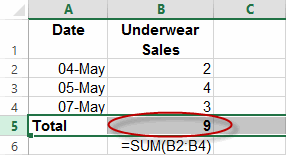
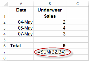
First I was going to show how SUM doesn’t handle row insertions immediately above the SUM function itself. So I duly made up a crappy example (if you’ll pardon the crappy pun):

…and then did the screenshot of the row insert, that showed how the formula didn’t adjust:

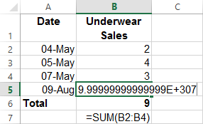
…and then went to add some ridiculously large number of underwear, for readers who need some point laboring:

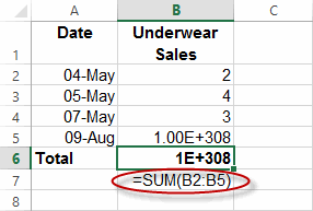
…and then pushed enter, and to my amazement saw that my example of “broken” ain’t, no more:

How utterly inconsiderate of Microsoft to fix this. Ruined a perfectly good example that I figure I could have dragged out for another half a chapter. Bugger! Now I have to write something else. God I hope they don’t fix the CONCATENATE function before I finish the book, or I’m screwed.
Edit
I just heard from Bill Jelen, who mentions when this gets autocorrected in this really great podcast of his:
He says “Going back to Excel 2003, provided you have a series of three or more numbers, Excel’s going to rewrite the formula to handle the new rows”.
But do check out that link: It’s hilarious. Also check out the follow-up podcasts.
There’s nothing like an Excel nerd with too much time on his hands…
I just tested your scenario in 2010 and 2007. The formula corrects itself in both those versions as well.
For some reason, I’ve never trusted that automatic stuff though. I have my method of always inserting the row in the middle of the range, which causes complications if I’m trying to maintain a certain order. Or, my preferred method is to use the table feature wherever possible. I trust that to maintain any dependent formulas.
Thanks Omar. I just heard from Bill Jelen, who mentions when this gets autocorrected in this really great podcast of his:
https://youtu.be/O-b8PjQ5_Nc
He says “Going back to Excel 2003, provided you have a series of three or more numbers, Excel’s going to rewrite the formula to handle the new rows”.
But do check out that link: It’s hilarious. Also check out the follow-up link at https://www.youtube.com/watch?v=BFa9vB1oljU
Funny link. Ad agencies have a hard time selling to knowledgeable customers. My industry is to sell to farmers. Ad agencies like to flip photos to get the right layout. That is really obvious to any farmer whenever a machine is involved.
I did a further test. I moved the AutoSum created formula to another sheet. Then did the insert row thing. The formula did NOT update to the extended range. Now I remember why I learned to never trust this “feature”. It fools you into thinking you are okay, but “out of sight” formulas are now broken.
I’m with Omar on this, I don’t like or trust this feature at all (and thanks for the reminder to switch it off on my new machine).
If the formula was adjusted when the row was inserted, that would be OK (maybe), but leaving the formula adjustment until a number is entered in the blank cell I don’t like at all. To make matters worse, it’s inconsistent in how it handles non-numeric data that is entered and deleted, or copy and paste data.
More details at: https://newtonexcelbach.wordpress.com/2009/04/20/a-very-un-useful-feature/
To quote from that post: The solution is simple; go into Options-Advanced and unselect the “Extend data range formats and formulas” feature.
Thanks for the link, Doug. Now I’ll put that half chapter back in.
Yeah, who types in numbers anyway? Isn’t almost everything just copy/paste? But seriously, in anything more than the most trivial spreadsheet model there are way too many numbers to manually key in. They’ll either be pasted from elsewhere or formula driven referencing another sheet or cube functions. Copying the formulas down doesn’t trigger the range extension either. No wonder I’ve never seen the formula range extend automatically.
To me, the CellAbove is really useful in another context: In tables!
1. Performance optimization: Really often, the table is sorted by multiple dimensions. So instead of using a VLOOKUP (or INDEX/MATCH) in each row, I rather have one column that depicts if it is the same category as the row above, eg.:
(I know, I could define a name CityAbove as $B1 but that would be overkill IMO). Then the formula for Population would be something like
.
2. Construction of “leaping counters”: Rather often I I find myself in need to re-arrange data, e.g. normalizing/unpivot a value copy of a pivoted data. While this can be done many ways (I now mostly use PowerQuery for this), one way is a table with two “counter columns” – Row and Column. For this, I would define
and
. (The N function is used to convert the table header to 0). Now, I can easily translate the cross-tabbed data with
Jef, do I understand this correct? Do you use examples of tables in your book that are NOT formatted as tables? Please tell me I’m wrong. Please…
I don’t use tables that are not formatted as tables. So in those screenshots, there is not a table in sight. I do make heavy use of tables throughout the book. Just not in that particular example. And if I use that particular example above, I’d probably say “Why bother with this, when you can use a table and just sum the table reference”.
For those still using pre-2013 Excel, enter this formula in the total row (A10) to sum the range A1:A9 and not get burned by the insert row problem.
=SUM(A1:OFFSET(A10,-1,0))
@Jorma: Problem with OFFSET is that it’s volatile – which can be rather painful in complex workbooks (see http://www.decisionmodels.com/calcsecretsi.htm). Better use a proper Excel table and the formula
To avoid the volatil OFFSET
=SUM(A1:INDEX(A:A,ROW()-1))
Regards
I realise in hindsight that the cellabove trick IS still needed, because it still works in the event that say a calculated column formula references a cell in the previous row, and a user inserts or deletes a row. With traditional relative references, you’ll get a REF! error. With CellAbove, no error.