Filtering PivotTables with VBA? Deselect Slicers first!

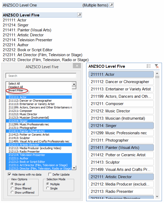
I’m in the final stages of coding up a commercial add-in that gives you lot more filtering options for PivotTables at your fingertips than you get out of the box. Here’s how it looks, along with the PivotTable its connected to and a native Slicer for comparison:
 
Pre Invert


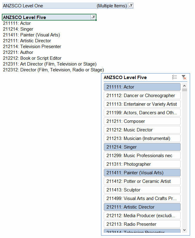
As you can see, it offers you a lot more tricks than a native Slicer – including a nifty ‘Invert Filter’ function. It also lets you see a lot more items displayed in it compared to a Slicer: 22 items are visible in mine, vs just 17 in the correspondingly sized Slicer. And that’s one of the many beefs I have with Slicers…they take up far too much screen real estate for the scant options they offer. In fact, my version takes up no screen real-estate most of the time: it launches simply by double-clicking the PivotTable field header, and you can dismiss it when you’re done to free up space if you want:
 
Slicer Dismissed
 
 
So about that Invert Filter function. I love clicking on that sucker over and over again. It takes about 7 seconds to invert my sample PivotTable that has 1000 items in it (12 items of which are selected in this example). That’s actually pretty fast as far as inverting a PivotTable, because you need to change the .visible status of all 1000 PivotItems, and as per a previous post that’s very slow to do unless you get tricky. And 7 seconds is a vast improvement on the method Microsoft gave you…none. I can’t comprehend why simple options like these are not built in to Slicers and Tables, but your filtering pain is (hopefully) my financial gain. (Yep, this works on Tables too.)

If I click that Invert Filter label, then here’s the after-effect:
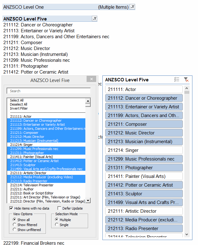
 
Inverted


Beautiful: 7 seconds, and she’s turned completely inside out. Unless that is, that Slicer happens to be selected. Then it takes a full minute. Why? No idea. Moral of the story: if you’re writing code to filter PivotTables, then you probably want to make sure any Slicers for that field are deselected first. Not disconnected…you can leave ’em in place quite happily, and the code won’t suffer.

Anyways, that’s the first look at my new baby. It does a lot more than just this inverting trick, too. Among other tricks, it lets you filter PivotTables based on external ranges, and gives you some absolutely fantastic new tools for filtering PivotFields based on just about any tricky search conditions you might want to string together – but that’s a subject for my next post.
Excel User Voice and Workbook Calculate

Excel User Voice

At the recent Excel Global Summit the Excel team were keen to explain how they have started using Excel User Voice to ask for and prioritise product improvement suggestions.

https://excel.uservoice.com/

There are 2 important things to note about this:

  1. The Excel Dev Team actually read your suggestions on User Voice!
  2. Starting with Excel 2016 the development and ship cycle is much much faster than the traditional 3 years.

So it really is worthwhile making your suggestions to improve the product.
You get 10 votes on suggestions, and the suggestions are categorised by end-point and product area. So if you want to make a performance suggestion for Excel on Android phones you can focus down, see what other suggestions have been made in this area, and either cast a vote for an existing suggestion or make a new suggestion.

Workbook Calculate

To try this out I made a suggestion (about calculation of course).

At the moment from the UI you can either calculate all open workbooks (F9 or Automatic) or a worksheet (Shift F9).
From VBA you can also calculate a range (Range.Calculate and Range.CalculateRowMajorOrder).

But you cannot calculate a single workbook.

This is really annoying when you have 2 versions of a large slow workbook open, or you have a small rapidly changing workbook open that links to a large mostly static workbook.

My suggestion is to add an additional calculation setting: Calculate Active Workbook Only and from VBA Workbook.Calculate.

https://excel.uservoice.com/forums/304921-excel-for-windows-desktop-application/suggestions/10601079-workbook-level-calculation

So please vote for my suggestion if you think it’s a good idea!

Listbox bulk refresh won’t redraw if called by Listbox click.

I’ve been playing around with ListBoxes recently. Or more to the point, they’ve been playing around with me. After much staring and swearing, I’ve found that you can’t get a ListBox to repaint itself when feeding it an entire list in one go in response to a Listbox_Click event in that same ListBox. It does however repaint correctly if you run the exact same code from somewhere else…say a CommandButton-initiated action.

By new list, I’m talking about populating the ListBox with an array via the Listbox.list=SomeArray approach. The .AddItem method works fine. So there’s always that: you can simply remove all items one by one, then add all the new items one by one. But that’s really slow: on my laptop it takes something like 15 seconds to add 10,000 items to that listbox. And it gets slower the more you add. And you can probably double that, if you need to replace each and every one of those items with something else. Whereas the Listbox.list=SomeArray approach takes less than a second to add ten times as many items. It’s fast.

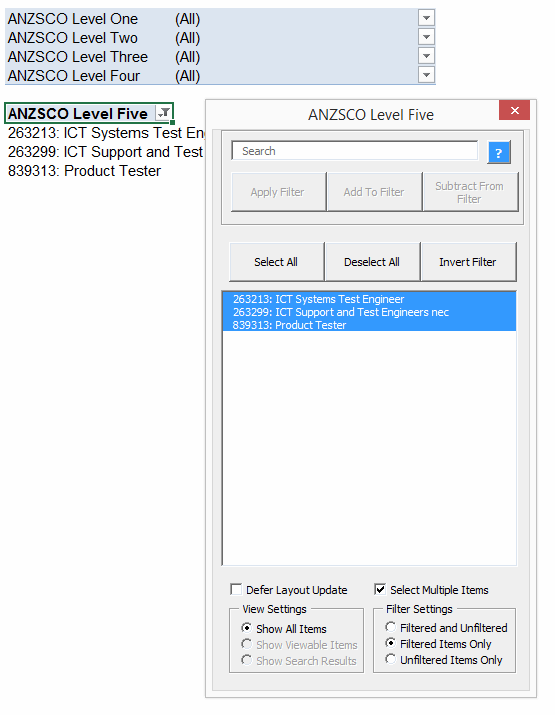
So why would you want to add tens of thousands of items to a ListBox? And why would you want to perform a wholesale update that list by clicking in the Listbox itself? Here’s why: I’m designing a UserForm to help filter PivotTables. It’s a cross between the existing Pivot Filter functionality and a Slicer. Here’s what you see if you double-click on a PivotField header:

Initial State

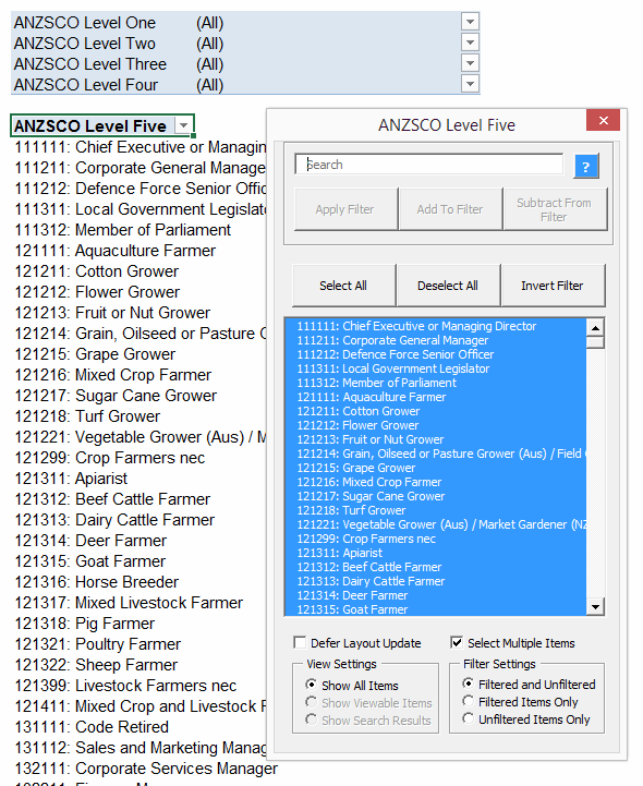
Note the Search field at the top, and the three buttons immediately below that search field. If you type something into that field, then instead of displaying everything that’s currently filtered, you instead get a list of any matches, and you can then apply those search results to the underlying PivotTable via those three CommandButtons. The first cb simply filters the PivotTable to reflect the search, and the other two let you add or remove any search result from an existing filter. (The native filter lets you add, but not remove).

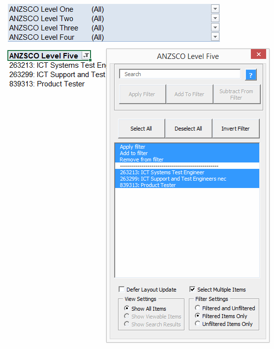
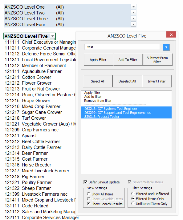
I want to do away with those three command buttons, and instead (in the event that a search is performed) simply list those three options at the top of the ListBox above any search results returned. Clicking on those three options will then trigger the exact same code as currently triggered by the Command Button.

Here’s how that looks currently if I actually type something in that Search box (Note I haven’t yet removed the three command buttons this new functionality will make redundant from that Search frame):

test search

I’ve added a simple bit of code to the lbResults_Change() event handler that checks if a user clicks any of those first three options. All that code does is trigger the exact same routines as would be triggered if they’d simply clicked on the actual command buttons themselves:

The listbox gets updated just fine if I click on the command buttons, as you can see from the below. The Pivot has been filtered accordingly, and those contextual search options have been removed from the top of the listbox (and the search field cleared):

CB press

But watch what happens if I trigger the exact same code by clicking that first option in the ListBox itself:

ListItem

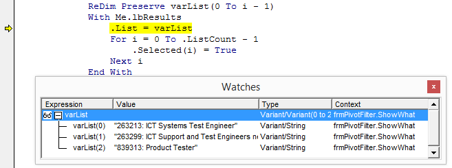
As you can see from the above screenshot, it still shows those three options at the top, even though they are NOT in the array that I assigned to the listbox, as evidenced by the screenshot below:

Watch

The Listbox DID get updated, mind:

…It just didn’t get redrawn. And it won’t get redrawn unless I refill the ListBox via one of those CommandButtons I’m trying to do away with. And it doesn’t seem to matter if I set the focus to the CommandButton before I try to refresh the Listbox, or even clear the ListBox entirely before I try to refresh it.

You can see this behavior for yourself in this sample file I’ve prepared.

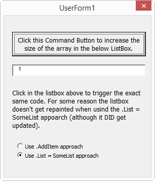
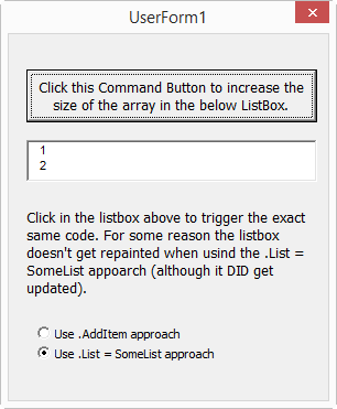
When the userform opens, you’ll see this:

Userform1

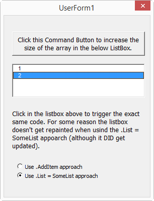
Clicking the CommandButton correctly loads a new array into the ListBox (and increases the size of the ListBox accordingly):

Userform2

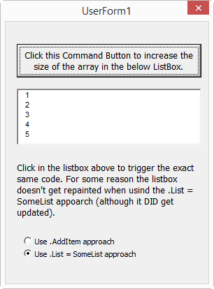
…but if you click in the ListBox itself – which triggers the exact same code – then while you’ll see that the ListBox got expanded, it did not get redrawn:

Userform3

Just as weird: you can see that the ListBox got expanded by two lines. That’s because the ListBox_Click event got executed twice…even though I have the requisite event suppression code in place (and I’m not talking about application.enable events here, because that doesn’t work for UserForm events). Putting a breakpoint in the code also shows that the 2nd time it runs occurs immediately after the previous run finishes, and not as a response to the .list = SomeList bit that normally triggers such repeat runs.

And if I now click that CommandButton, you can see that the missing numbers from the double ListBox_Click pass are in fact there, as well as the extra addition from the latest CommandButton_Click:

Userform4

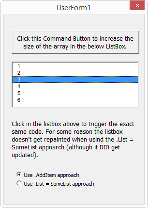
If I click that Use .AddItem Approach radio button and then click in the ListBox, things go according to plan:

Userform5

So there’s always that approach. But that approach sucks. Maybe I’ll be forced to keep those CommandButtons in the UserForm after all. Anyone else experience this issue, or have a workaround up their sleeve?

Happy Gerbitz Day

This is the first year you can sing “Happy Birthday” to Excel without having to pay a royalty, so that’s nice.

Here’s my uninteresting Excel story: My first spreadsheet program was SuperCalc. I remember we had orange screens on our PCs. Eventually we graduated to VGA monitors and Lotus 1-2-3 v.1A. I stuck with that version for a long time. I had tons of keystroke macros – whatever the heck those were called in Lotus – and I wasn’t giving them up. Excel burst onto the scene and I barely blinked. I don’t need that fancy new stuff. I used v.1A until 1992 and I think 1-2-3 was on v4 by then.

In 1992, I miraculously got a job at KPMG (nee Peat Marwick). Apple was a client of KPMG, so everyone got a Mac and used Office. It was like living in hell. I was a PC, Lotus 1-2-3 guy and I was forced to use these toys in business. Over time, I got used to my Mac Plus, then my SE30, then my PowerBook. And, of course, I got used to Excel and its obviously superior features to the version of 1-2-3 I was using. I don’t remember what version of Excel that was, I just know that most people in my office sucked at using it. Thankfully 25 years later, every office worker is, at a minimum, competent at Excel. What? That’s not true, you say? There are still people who work with Excel and aren’t competent? What the hell have they been doing for the last 25 years? It’s not like learning Excel is exactly cutting edge. End rant.

Being forced to use Office was probably a pivotal point in my life. (Using Macs in an accounting firm in the early ’90s was just stupid.) Pivotal though it was, I think what really turned me into an Excel geek was an intranet message board that KPMG had. I think they called it the KPMG Knowledgebase, but my memory isn’t so good. I could go on the message board and answer people’s questions about Excel. And I was hooked. Then it was on to newsgroups (nntp), a blog, and the crazy post-Microsoft newsgroup period that has mostly meant StackOverflow.com for me. What the heck did I do after MS closed the newsgroups but before SO? I don’t remember. I know I visited answers.microsoft.com once, saw a terrible answer from a moderator, and saw that the moderator had selected his own answer as “the” answer. I haven’t been back.

When I first started on the newsgroups, I was more of an Access guy than an Excel guy. I was surely answering more Access questions than Excel at the beginning. It was when I started reading Chip Pearson, Rob Bovey, Stephen Bullen, and others posting about VBA that the tables turned. I realize that Access has VBA, but the Excel object model was, and is, a thing of a beauty. I still do plenty of Access work, but it pales in comparison to the time I spend in Excel.

Other random memories:

  • At my first MVP Summit, everyone thought I was going to be a 60-year-old guy and I was in my mid-thirties. I guess I came off as cantankerous mature in my newsgroup postings.
  • I remember after a year of DDoE, a bunch of fellow Excellers joined as authors. There were some great posts back then.
  • I remember applying for a job and taking an Excel and an Access test. I aced them both. The secretary was looking at me like I was a witch. (If you’re reading this blog, you could ace them too.)
  • I remember planning an Australian Excel conference over beers and actually going through with it. If I had a nickel for every plan I made over beers that came to fruition, I’d have a nickel.

Warning: Special Cells slows to a crawl across multiple columns

Further to my previous post on Goto Special/Blanks, it looks like there is a pretty serious problem with the SpecialCells method if you use it on more than one column.

That’s because it’s blindingly fast at finding things in one column, but painfully slow in finding things in any other columns. Which is a problem, because anyone who’s anyone knows that using SpecialCells is supposed to be much more efficient than looping through a big range. Well, Mr and Mrs Anyone may want to reconsider using the loop on multiple columns. Or rather, they might want to consider looping through the columns, and use SpecialCells on each one individually. Best of both worlds.

So how fast is it on one column? And how slow on multiple columns? Let’s find out.

Here’s your test code.


Sub TestingTestingIsThisThingOn()
Dim TimeTaken As Date
Dim rng As Range
Dim Jeff As AboveAverage

TimeTaken = Now()
Set rng = Range(“A:B”)
rng.SpecialCells(xlCellTypeConstants, xlTextValues).Select

TimeTaken = Now() – TimeTaken

Debug.Print “UsedRange:” & vbTab & ActiveSheet.UsedRange.Address
Debug.Print “Range Searched:” & vbTab & rng.Address
Debug.Print “Time Taken:” & vbTab & Format(TimeTaken, “HH:MM:SS”) & ” seconds.”
Debug.Print “Cells: ” & Selection.Cells.Count & vbNewLine & vbNewLine
End Sub

Fill A:A with some text, such as “Blindingly Fast”, and run that sub. Here’s what I get:

UsedRange: $A:$A
Range Searched: $A:$B
Time Taken: 00:00:00 seconds.
Cells: 1048576

Now fill B:B with “Painfully Slow”, and run it again. Here’s what I get:
UsedRange: $A:$B
Range Searched: $A:$B
Time Taken: 00:02:02 seconds.
Cells: 2097152

What the…? So it took a blindingly fast 1 second to process one column, and a painfully slow three minutes to process two? That’s about as linear as my life story before I met and married Excel 2000. (My first wife. I still see her round from time to time in the forums. She hasn’t aged gracefully.)

So either there’s something SpecialCells doesn’t like about the number of columns, or there’s something it doesn’t like about the number 1048576. Let’s find out.

If you delete rows 524288 down, then you’re left with 2 columns of text totaling 1048576 cells. Here’s what I get if I run the code on that:

UsedRange: $A$1:$B$524287
Range Searched: $A:$B
Time Taken: 00:00:57 seconds.
Cells: 1048574

It took one minute to process this, as opposed to the one second it took to process the same amount of cells in one column. So it seems that it’s the multiple columns aspect that is causing the issue, and that the extra time incurred is dependent on the number of cells in that 2nd column. In fact, if I fill those blank cells in column A with our text (while leaving half of Column B with blanks) and rerun the code, then it doesn’t take Excel any longer to process those extra half million cells:

UsedRange: $A:$B
Range Searched: $A:$B
Time Taken: 00:00:52 seconds.
Cells: 1572863

So it seems the issue is in how Excel is handling the union of all those cells it identified in the first column with any cells it identifies in the second. And given how slow it is, I wouldn’t be surprised if it’s unioning those cells one at a time.

The same thing goes for blanks, by the way. This turned up in the comments of Doug Jenkin’s latest post.
Moral of the story: Do NOT use SpecialCells on more than one column at a time.

Question: How are you supposed to bring this stuff to MS’s attention, apart from posting it somewhere conspicuous like here?

—Update—

Over in the comments of his blog, Doug Jenkins hypothesizes:

A possibility is that a single column is treated as being a single array with 1 million values, but two columns are treated as being 1 million arrays, each with 2 values. When the operation is done on the spreadsheet with F5-Special, the name box shows that it works row by row, rather than all of Col A then all of Col B.

I think he’s right. And also after further testing, I realize that those times are down to how long Excel took to search all these arrays, and not to do with how long it took Excel to union the results. Because there weren’t that many results to union in my simple example, so it took practically no time at all.

But if you set up the data like so:
 
Every 2nd blank
 
 
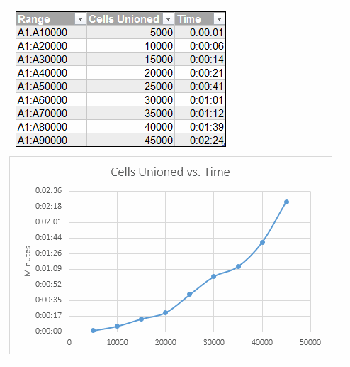
…then you see that the actual unioning takes a heck of a lot longer than the searching. For instance, as per above it took nearly two minutes for SpecialCells to search 1 million rows across two columns and identify a handful of blank areas. Whereas from the below table, you can see that with the greatly increased number of blanks that it’s got to union, it took over two minutes to union just 45,000 cells in one column.
 
Results

What good is the Data Model without PowerPivot?

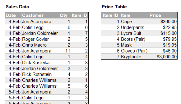
So in the book I’m forever writing, I have an example of how you can use the Data Model to effectively do VLOOKUPS. Take the example where we’ve got a transactional list of sales that has a product ID but no ‘friendly’ name or price, and another table that maps Product ID to price and friendly name.
 
Two tables
 
 
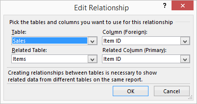
We can use the Data Model to set up a relationship between these two tables…
 
Edit Relationship
 
 
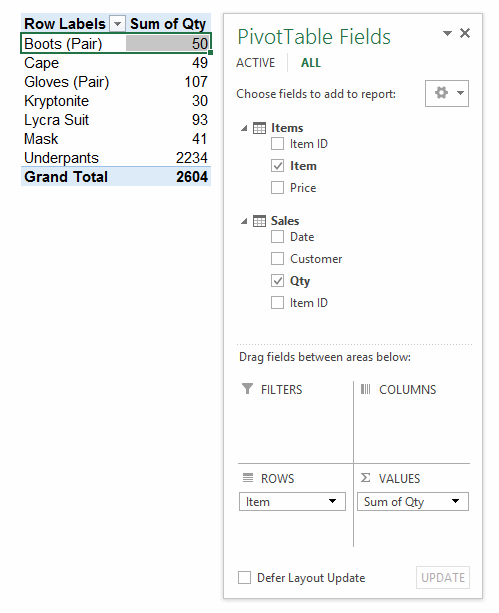
…so that we can display friendly product names from the Price table against aggregated sales quantities from the Sales Data:
 
PivotTable1
 
 
Sweet. No VLOOKUPs necessary. So…given that we’ve got quantity, and prices, how much money did we make? Let’s find out. First, lets’ drag that Price field into the Values area of the PivotTable and see what it gives us:
 
PivotTable2
 
 
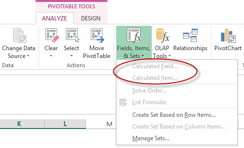
Well, that obviously isn’t what we’re after…it gives us the price of every item, not total revenue. Maybe we need to create a calculated field to multiply Qty against Price:
 
Calculated Dialog
Oh wait…we can’t. Unless the average user has a premium version of Excel that includes the glorious thing that is PowerPivot (not to mention the wherewithal to not be daunted by a completely different, programmer-centric User Interface) then they can’t do this rather basic datamodel-ish thing.

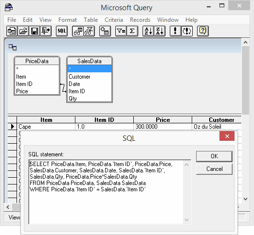
So here we are…15.64% of the way through this century, and yet your average user still doesn’t have the ability to mash together relational tables in the world’s most widely used business productivity tool. (Or mash together flat files from different sheets or workbooks, for that matter.) Unless of course they go back to last century and do it like this:
 
ms query
 
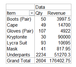
Query Pivot
 
 
I just don’t get this. What’s the point of exposing non-premium users to something like the Data Model if it doesn’t let them do diddly squat? Without calculated fields, surely it’s a big red herring that unnecessarily confuses users? (And okay, so if the Data Model on its own isn’t the hammer for this particular nut, what is?)

I thought I was missing something here, so asked someone smarter than me about these matters (Sam). Sam tells me:

From 2013 onward the Data Model and the DAX Engine are separate
The Data Model is only to create Relationships (Joins) – available to all versions of Excel. The DAX engine if for the Calculations – the Pro Plus and Stand Alone versions.
The only extra function on which you can aggregate data in the Data Model based Pivot Table is Distinct Count at the expense of Numerical Count and Product of a normal pivot. A Data model based pivot table disables both Calculated fields and Items as well as the ability to Group. So the short answer is No – you need DAX alternately use SQL to create the Joins

Don’t get me wrong…Powerthis and Powerthat is all very exciting. But Microsoft: How about showing the tiniest bit of love for the common man (and woman) who live in the common version. Those folk shouldn’t have to upgrade to some fully-featured business intelligence flagship product merely so they can mash data from within Excel together, surely? (And yes, they might be able to use PowerQuery for free to join their relational data together, but leaving aside the fact that they’d probably end up with a flat file in Excel after importing the data from PQ, it’s just not good enough that they would have to go learn another programmer-centric tool just to do something that should be childs-play in Excel itself. )

Just to be clear, I’m not one of those that think that PowerPivot should be bundled into all versions of Excel just because we want it to be. Microsoft have spent a lot of money on PowerPivot, and I don’t expect them to have a sudden attack of benevolence merely because it suits users. Theirs is a money-making venture. And their shareholders expect them to do the best job possible at that. But here’s the thing: It’s nearly 2016, and MS still have not given users the ability to do some pretty basic stuff natively in Excel, such as mash together data in separate sheets or workbooks and serve it up piping hot as a PivotTable. Don’t they know that in the real world, people have to mash together data from different sheets all the time? You get a sheet emailed to you from division A, a sheet from division B, and a sheet from division C. You need to mash it up to get an overview. A lot.

I’m not asking for Tableau here. I’m just asking for a core product that also moves with the times. Or at the very least, keeps up with last century.

Easy way to back up CF formats

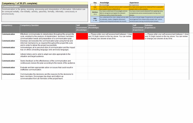
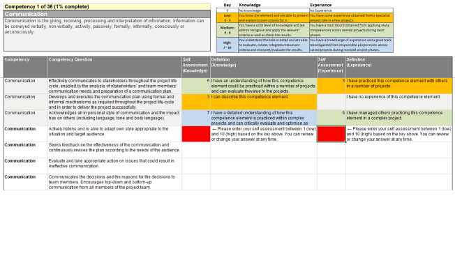
I’m working on an application that Project Managers use to test their competencies against a competency framework. There’s a lot of questions and I don’t want to freak them out by showing all at once, so I use Conditional Formatting to unhide the questions in batches, as well as to highlight the next thing that needs to be answered, and to show how their self assessment corresponds to the ratings key.

Here’s how it looks before users start filling it out: only the first batch of questions relating to the first competency area are displayed:
 
Comp blank_Small
 
 
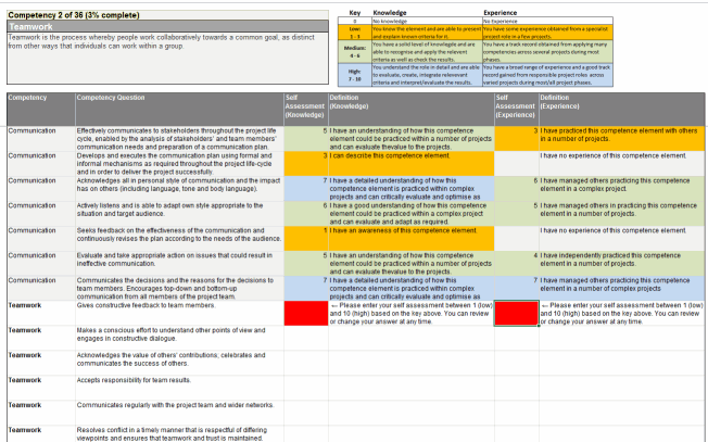
As they complete it, their answers get color-coded to match the key:
 
Comp Partial_Small
 
 
When they complete the last question in regards to the current competency they’re working on, the next batch of questions for the next competency appears, and the definition for that competency overwrites the previous one in the top left:
 
Comp next_Small


I’m using CF because I don’t want to use code to do this if I can help it, so I don’t have to deal with security settings or questions about enabling macros. Plus I’m just there for 4 weeks, and there isn’t going to be a VBA developer picking up the project after me.

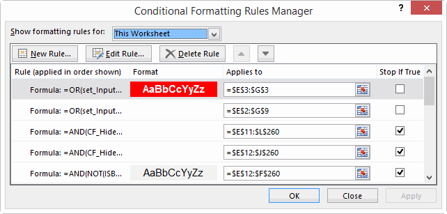
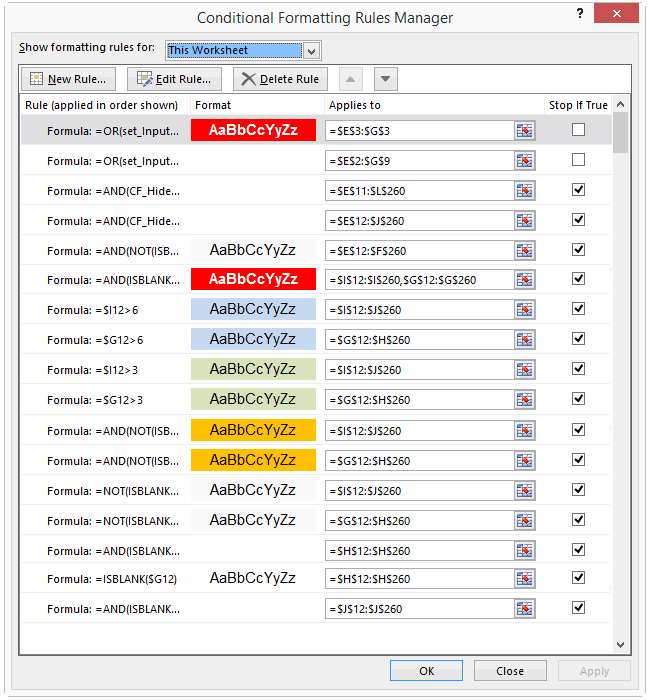
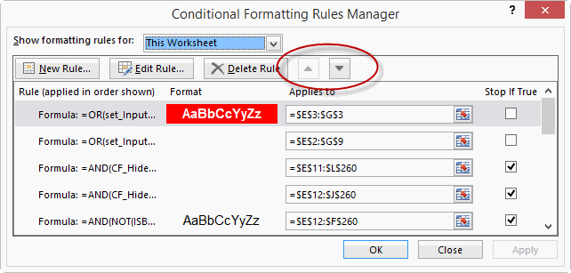
But the CF dialog – how shall I put this delicately – seems as if it was built by Microsoft. (Ok, so I threw tact to the wind there. It’s a dog, a pig, and a slug, all rolled into one needy, dirty, slimy son-of-a-bitch pest.) Here’s all it shows me in all of its non-resizable gory. (Yes, gory, not glory.):
 
CF Manager
 
 
Using it is like trying to build a ship in a bottle inside of another ship in a bottle. Now I know how proctologists feel. If it was half the dialog box that the Name Manager was, it would at least yet you resize so you could see all your conditions at once:
 
Slightly better
 
 
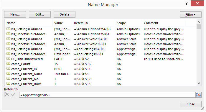
Just look what the Name Manager gives us, by way of comparison:
 
Name Manager
 
The Name Manager gives us friendly names, notes where we can record what does what, resizable columns, and a resizable dialog. Compared to that, the CF dialog is like the punchline from a Monty Python skit.
 

“Oh, we used to dream of having a resizable dialog box.”
 
 
What’s worse, I keep noticing that the order of my CF conditions gets scrambled – maybe when I copy the sheet to a new template, maybe when I insert or delete columns, maybe when I don’t look suitably impressed whenever it does work correctly. I don’t know.

So I thought I’d look for a way to back them up. I looked at Dicks’ posts Listing Format Conditions and Listing Format Conditions Redux, but those would need more work still in order to record the formatting, and then a routine to restore everything from the storage table.

But then I discovered this: If you fire up the macro recorder, bring up the CF dialog box, select Manage Rules, select Show formatting rules for This Worksheet, and then makes some trivial change – such as click the down arrow to move the currently selected CF condition down one, then click the up arrow to put it back:
 
CF Manager_Move
 
 
…then as soon as you push OK the Macro Recorder spits out a macro that clears all the format conditions on the entire sheet, and then builds those CF rules again from scratch. All of them. Here’s an excerpt:


Sub Macro7()
Cells.FormatConditions.Delete
Range("PM[Definition " & Chr(10) & "(Experience)]").Select
Range("G14").Activate
Selection.FormatConditions.Add Type:=xlExpression, Formula1:= _
"=AND(ISBLANK($I14),$T14=FALSE)"
Selection.FormatConditions(Selection.FormatConditions.Count).SetFirstPriority
With Selection.FormatConditions(1).Font
.ThemeColor = xlThemeColorDark1
.TintAndShade = 0
End With
Selection.FormatConditions(1).StopIfTrue = True
Range("PM[Definition " & Chr(10) & "(Knowledge)]").Select
Range("G14").Activate
Selection.FormatConditions.Add Type:=xlExpression, Formula1:= _
"=ISBLANK($G14)"
Selection.FormatConditions(Selection.FormatConditions.Count).SetFirstPriority
With Selection.FormatConditions(1).Interior
.PatternColorIndex = xlAutomatic
.ThemeColor = xlThemeColorDark1
.TintAndShade = 0
End With
Selection.FormatConditions(1).StopIfTrue = True

End Sub

That – my friend – is your CF backup. The only thing wrong with this code is that it keeps putting the line Range(“G14”).Activate in the middle of each block for some strange reason. That happened to be the cell I had selected when I recorded the macro. But if you do a find and replace on the code to ditch it in favor of a more helpful “” then the code works fine. (Yes I know that CF is relative, but that’s still no reason why it should select the cell I have selected and then apply the formatting to it rather than to the desired target). (Edit: You need this activation if you are dealing with CF conditions with relative referencing. But it doesn’t work properly in the event that you originally applied CF to a range while you had another range outside of that CF area selected. The CF manager takes account of this properly, but the macro output doesn’t, meaning it selects a range, then activates a cell/range outside of that selection, which screws things up. So it pays to eyeball the code for situations like this.)

Now what would be cool is if someone out there was to code up a routine that uses extensibility to read this from the VBE and populate a handy table in the worksheet with all the parameters. Extra credit to someone who devises a way to make the macro recorder fire up and do this automatically for each sheet.

Even better: it would be amazing if Microsoft would show the CF dialog the slightest amount of love. CF could be one of the most powerful features of Excel for non coders. But not as it stands at the moment. Right now, it’s a pigdogslug.

An even easier way

So I got to thinking that if Excel will quickly spit out a complete list of FormatConditions at the ‘AppliesTo’ level for the sheet, it must have them stored in a collection somewhere. And that collection is…drum roll please…the Cells object.

Want some code to quickly and easily print out every format condition everywhere? Here ’tis:

Sub FindCF()

'We have to Dim WhatIsIt as a generic Object instead of declaring as FormatCondition because DataBars screw things up.
'See http://excelmatters.com/2015/03/04/when-is-a-formatcondition-not-a-formatcondition/

Dim WhatIsIt As Object
Dim fc As FormatCondition
Dim db As Databar
Dim cs As ColorScale
Dim ics As IconSetCondition

Dim ws As Worksheet
For Each ws In ActiveWorkbook.Worksheets
For Each WhatIsIt In ws.Cells.FormatConditions
Select Case TypeName(WhatIsIt)
Case "Databar":
Set db = WhatIsIt
Debug.Print "Type: " & "DataBar" & vbTab & "Applies To: " & db.AppliesTo.Address
Case "FormatCondition"
Set fc = WhatIsIt
Debug.Print "Type: " & "FormatCondition" & vbTab & "Applies To: " & fc.AppliesTo.Address & vbTab & "Formula: " & fc.Formula1
Case "ColorScale"
Set cs = WhatIsIt
Debug.Print "Type: " & "ColorScale" & vbTab & "Applies To: " & cs.AppliesTo.Address
Case "IconSetCondition"
Set ics = WhatIsIt
Debug.Print "Type: " & "IconSet" & vbTab & "Applies To: " & ics.AppliesTo.Address
Case Else
Stop
End Select
Next WhatIsIt
Next ws
End Sub

Code? Luxury!

Global name meets Local, Global freaks out

So here’s something I came across today. Somehow I’d managed to set up both local AND global names in a sheet, and found that I pretty much couldn’t do anything with the Global name via VBA as a result.

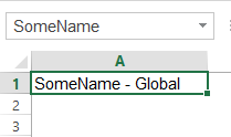
Say I set up this global name:
 
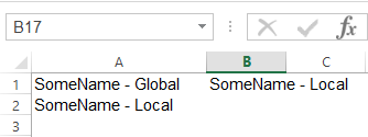
SomeName - Global
 
 
Note that it says SomeName in the NameBox when I have the name selected. Nothing weird about that.

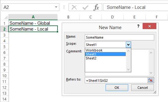
Now I add a local name with the same name, pointing to A2:
 
SomeName - Local
 
 
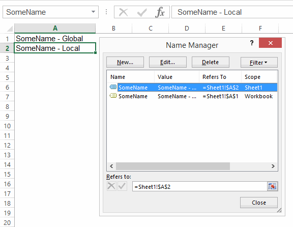
…and here you can see both names in the Name Manager. Note that it says SomeName in the NameBox when I have the local name selected. Nothing weird about that, either…local names take precedence over global.
 

SomeName - Both_Name Manager
 
 
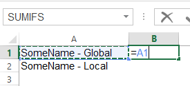
If I type = then select A1 where the global name lives, note that no name comes up in the intellisense:
 
Equals Global
 
 
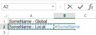
..but if I do the same with the local name, I get intellisense:
 
Equals Local
 
 
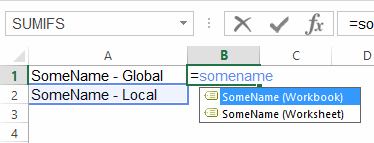
Now things get a little weirder. If I type =SomeName, I get two options in the intellisense:
 
Equals SomeName
 
 
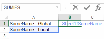
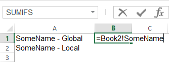
If I select the SomeName (Workbook) option, Excel qualifies the reference with the workbook name:
 
Book2 SomeName
 
 
…but when I push Enter, it’s still the local name that’s being referenced:
 
Book2 SomeName Not
 
 
…and when I select it again, I see that Excel has bizarrely changed that Book1! qualifier to a Sheet1! qualifier. In other words, it’s said ‘I know you asked for workbook, but I’m giving you local’:
 
Book2 SomeName Local Qualifier
 
 
So what the hell is the point of those two options in the intellisense, if no matter what you do, Excel gives you the local name? Beats me. What’s worse, if your workbook name has a space in it, then Excel forgets to wrap apostrophes around it, and the Update Values dialog comes up:
 
Update Values dialog
 
 
What a mess. Push cancel, and you’re left with an invalid name:
 
Book2 SomeName spaces


Names and Collections

It turns out that the local name gets added to both the ActiveWorkbook.Names collection AND the ActiveSheet.Names Collection:
? activeworkbook.Names.Count
2
? activesheet.names.count
1

You can reference both names by index number just fine:
? activeworkbook.Names(1).Name
Sheet1!SomeName
? activeworkbook.Names(2).Name
SomeName

…but any attempt to reference the globally scoped one by name gives you the local name. Here, I retrieve their names from their index numbers:
? activeworkbook.Names(1).Name
Sheet1!SomeName
? activeworkbook.Names(2).Name
SomeName

Here I retrieve their refersto ranges from those index numbers:
? activeworkbook.Names(1).RefersTo
=Sheet1!$A$2
? activeworkbook.Names(2).RefersTo
=Sheet1!$A$1

Here I try to retrieve their refersto ranges from their names:
? activeworkbook.Names(“Sheet1!SomeName”).RefersTo
=Sheet1!$A$2
? activeworkbook.Names(“SomeName”).RefersTo
=Sheet1!$A$2

And here I try to retrieve their names from their names:
? activeworkbook.Names(“Sheet1!SomeName”).Name
Sheet1!SomeName
? activeworkbook.Names(“SomeName”).Name
Sheet1!SomeName

As per this Stack Overflow thread, If you want to identify the global one, you have to loop through the collection of names and find the one that has an “!” in its name.

So there you have it: if you’re referencing names by name, don’t assume you’ll get the one you want. Tedious!