Here’s a funny little bug I came across today. So I’m adding a CF condition, and I push F3 to bring up Paste Names rather than type out a reference or name:
 

 
 
And clicking on that named range duly inserts it into my CF formula:
 

 
 
…but the only problem is, now I can’t seem to do anything else. I can’t type the closing bracket, because Excel won’t let me. I can’t backspace to remove the offending name, because Excel won’t let me. The cursor is still flashing, so Excel hasn’t hung.

If you type the name in manually rather than using F3, it works perfectly. It turns out its some kind of focus issue: if you push ALT + TAB the screen flickers, but you still have the Conditional Format dialog open and now it works perfectly.

It’s incredible what you can do with CF if you’ve got a good memory. The good memory bit is required because CF doesn’t let you write notes about what each condition does like Names do, or even assign those CF conditions meaningful names. Let alone (heaven forbid) resize the dialog box so you can see all your rules at once, to help you work out which does what:
 

 
 
With a good memory, it’s an incredibly strong and useful tool. With my memory, it’s downright mysterious.

Shame, because I’m using it to really good effect to steer users through a pretty complicated self-assessment tool. I pity the poor sap that comes after me that has to amend these rules. On the other hand, that poor sap will probably end up hiring me back at my urgent pickle rate. Thanks, Microsoft.

I was writing up the CellAbove trick for the book. You know, the trick outlined at Ken Puls’ place.

First I was going to show how SUM doesn’t handle row insertions immediately above the SUM function itself. So I duly made up a crappy example (if you’ll pardon the crappy pun):
 

 
 
…and then did the screenshot of the row insert, that showed how the formula didn’t adjust:
 

 
 
…and then went to add some ridiculously large number of underwear, for readers who need some point laboring:
 

 
 
…and then pushed enter, and to my amazement saw that my example of “broken” ain’t, no more:
 

 
 
How utterly inconsiderate of Microsoft to fix this. Ruined a perfectly good example that I figure I could have dragged out for another half a chapter. Bugger! Now I have to write something else. God I hope they don’t fix the CONCATENATE function before I finish the book, or I’m screwed.
 
 

Edit

I just heard from Bill Jelen, who mentions when this gets autocorrected in this really great podcast of his:

He says “Going back to Excel 2003, provided you have a series of three or more numbers, Excel’s going to rewrite the formula to handle the new rows”.

But do check out that link: It’s hilarious. Also check out the follow-up podcasts.

There’s nothing like an Excel nerd with too much time on his hands…

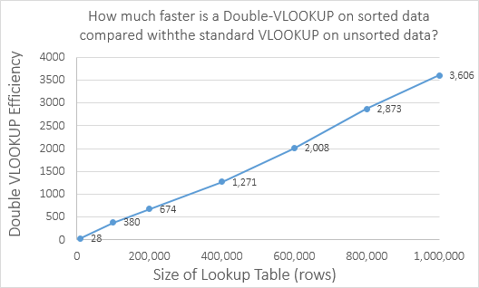
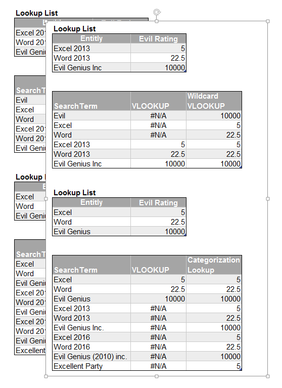
In my last post, I looked at how much faster the Double VLOOKUP trick was on sorted data compared with the usual linear VLOOKUP on unsorted data.

Below is the code for the timing routine I use. I stole the guts of it from joeu2004 who made some incredibly insightful comments at this great thread at MrExcel

If you’re going to time formulas, then that thread is required reading, because it makes this important point: we cannot always accurately measure the performance of a formula simply by measuring one instance of it. (But that does depend on the nature of the formula and the situation that we are trying to measure. Sometimes we need to measure one instance of a formula, but increase the size of ranges that it references in order to overcome the effects of overhead.)

I’ve assigned my code to a custom button in the ribbon. You just select the cells you want the formula to time, and click the button. (By the way, my upcoming book not only shows you how to do this, but also gives you routines for every one of the icons shown above and a lot more besides.)
 

 
 
In the above case, I’ve selected a 1 row by 3 column range. If your selection is only one row deep – and there’s more rows with data below – then the app assumes you want to time everything below too, up to the first blank cell it encounters. I may want to rethink that, but it works good for now.

And after I click the magic button, here’s the result:
 

 
 
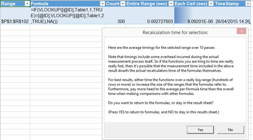
As you can see from the output screenshot above, it puts a new table in a new sheet, populates it with your timings and relevant parameters, and then displays a message with joeu2004’s warning in it. Plus – and I think this is the genius part – it lets you push OK to return back to the sheet where the original formulas are, or push Cancel if you want to stay in the output sheet.

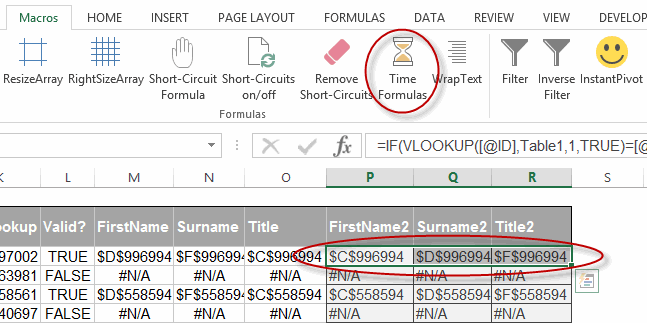
Note the ‘Formula’ column in the output table. For now, it just lists the formula that was in the top-left cell in the user’s selection. I think listing multiple formulas would be overkill. If there’s no formula in the top left cell, it sees if there’s a formula in the cell below. That way you can select headers in a Table, and you’ll still get the formula in the output.

It also can time multiple areas in one pass. So if I select that same range as a non-contiguous selection by holding Ctrl down and clicking each cell as I’ve done here (not that it’s easy to tell the difference visually from the previous screenshot):
 

 
 
…then here’s what I get:
 

 
 
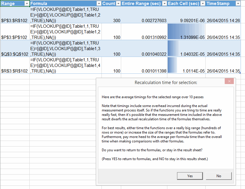
Man, that is sooo much better than having to do each formula separately and then having to manually copy the results from a messagebox into a Table, like I used to do.

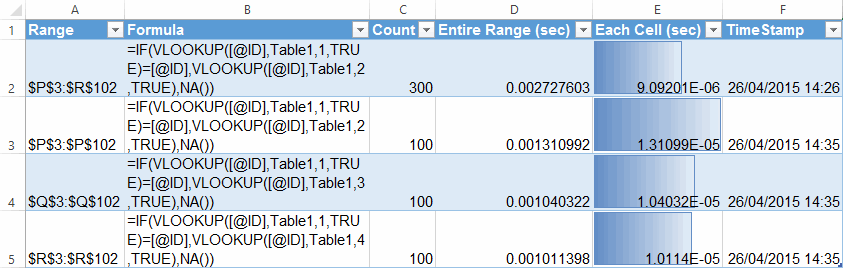
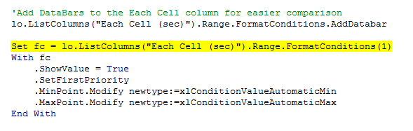
As you can see, I put a a databar on the important column, so you can visually eyeball results instead of conceptually juggling scientific notation in your head. But I’m damned if I can get this to display exactly as I want via VBA. For instance, here’s the databars I want if I add them manually:

Notice that those have nice borders, and sensible setting for the minimum values, meaning that first result also gets a databar. The code that VBA spits out when you add this default databar is pretty ugly:

Selection.FormatConditions.AddDatabar
Selection.FormatConditions(Selection.FormatConditions.Count).ShowValue = True
Selection.FormatConditions(Selection.FormatConditions.Count).SetFirstPriority
With Selection.FormatConditions(1)
.MinPoint.Modify newtype:=xlConditionValueAutomaticMin
.MaxPoint.Modify newtype:=xlConditionValueAutomaticMax
End With
With Selection.FormatConditions(1).BarColor
.Color = 13012579
.TintAndShade = 0
End With
Selection.FormatConditions(1).BarFillType = xlDataBarFillGradient
Selection.FormatConditions(1).Direction = xlContext
Selection.FormatConditions(1).NegativeBarFormat.ColorType = xlDataBarColor
Selection.FormatConditions(1).BarBorder.Type = xlDataBarBorderSolid
Selection.FormatConditions(1).NegativeBarFormat.BorderColorType = _
xlDataBarColor
With Selection.FormatConditions(1).BarBorder.Color
.Color = 13012579
.TintAndShade = 0
End With
Selection.FormatConditions(1).AxisPosition = xlDataBarAxisAutomatic
With Selection.FormatConditions(1).AxisColor
.Color = 0
.TintAndShade = 0
End With
With Selection.FormatConditions(1).NegativeBarFormat.Color
.Color = 255
.TintAndShade = 0
End With
With Selection.FormatConditions(1).NegativeBarFormat.BorderColor
.Color = 255
.TintAndShade = 0
End With


My code is just doing the first line:

'Add DataBars to the Each Cell column for easier comparison
lo.ListColumns("Each Cell (sec)").Range.FormatConditions.AddDatabar


…because no matter what I try, doing anything beyond merely adding the bars causes the code to error out. For instance, even if I just try and set the minpoint and maxpoint I get an error:
 

 
 
…and this successfully adds the min setting I want, but errors out when I try to add a listrow:
 

 
 
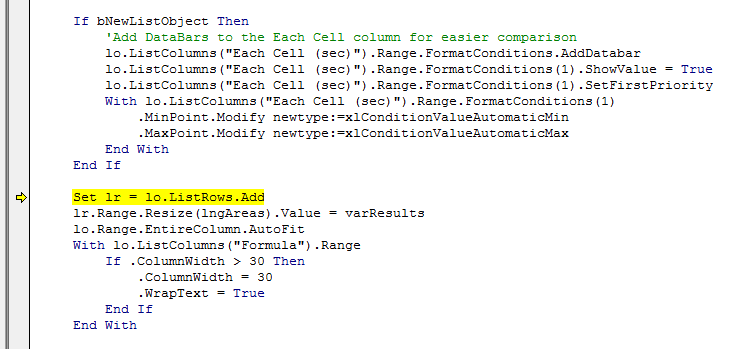
Even worse, when I end the routine, the screen no longer updates no matter what I do. So I have to close out of Excel entirely.

If anyone can tell me where I’m going wrong, I’d be much obliged. Might be another peculiarity of Excel Tables. Meanwhile, I’ll just run with those simple bars.

Here’s my draft code:

Option Explicit

Public Declare Function QueryPerformanceFrequency Lib "kernel32" _
(ByRef freq As Currency) As Long
Public Declare Function QueryPerformanceCounter Lib "kernel32" _
(ByRef cnt As Currency) As Long

'Code adapted from http://www.mrexcel.com/forum/excel-questions/762910-speed-performance-measure-visual-basic-applications-function.html
' Description: Determines formusa execution time
' Programmer: Jeff Weir
' Contact: excelforsuperheroes@gmail.com

' Name/Version: Date: Ini: Modification:
' TimeFormula 20150426 JSW Added in ability to record times to ListObject

Sub TimeFormula()
Dim sc As Currency
Dim ec As Currency
Dim dt As Double
Dim sMsg As String
Dim sResults As String
Dim i As Long
Dim N As Long
Dim oldCalc As Variant
Dim myRng As Range
Dim lo As ListObject
Dim lr As ListRow
Dim bUnique As Boolean
Dim strFormula As String
Dim myArea As Range
Dim lngArea As Long
Dim ws As Worksheet
Dim wsOriginal As Worksheet
Dim bNewListObject As Boolean
Dim lngAreas As Long
Dim varResults As Variant
Dim varMsg As Variant
Dim fc As FormatCondition

Const passes As Long = 10

With Application
.ScreenUpdating = False
.EnableEvents = False
oldCalc = .Calculation
.Calculation = xlCalculationManual
End With

Set myArea = Selection
lngAreas = myArea.Areas.Count
Set wsOriginal = myArea.Worksheet
ReDim varResults(1 To lngAreas, 1 To 6)
For Each myArea In Selection.Areas
lngArea = lngArea + 1
dt = 0
Set myRng = myArea
If myRng.Rows.Count = 1 Then
If Not IsEmpty(myRng.Cells(1).Offset(1)) Then Set myRng = Range(myRng, myRng.End(xlDown))
End If
N = myRng.Count
If myRng.Cells.Count > 1 Then
'Get formula from 2nd row in case we're dealing with multiple cells and happen to be on a header
If myRng.Cells(2).HasFormula Then strFormula = myRng.Cells(1).Formula
If myRng.Cells(2).HasArray Then strFormula = myRng.Cells(1).HasArray
End If

If myRng.Cells(1).HasFormula Then strFormula = myRng.Cells(1).Formula
If myRng.Cells(1).HasArray Then strFormula = myRng.Cells(1).HasArray

With myRng
For i = 1 To passes
sc = myTimer
.Calculate
ec = myTimer
dt = dt + myElapsedTime(ec - sc)
Next

'Record results for this pass
varResults(lngArea, 1) = myRng.Address
If strFormula <> "" Then varResults(lngArea, 2) = "'" & strFormula
varResults(lngArea, 3) = N
varResults(lngArea, 4) = dt / passes
varResults(lngArea, 5) = dt / N / passes
varResults(lngArea, 6) = Now
End With

Next

bNewListObject = True
For Each ws In ActiveWorkbook.Worksheets
For Each lo In ws.ListObjects
If lo.Name = "appTimeFormulas" Then
bNewListObject = False
ws.Activate
Exit For
End If
Next
Next

If bNewListObject Then
Set ws = ActiveWorkbook.Worksheets.Add
On Error Resume Next
ws.Name = "TimeFormula"
On Error GoTo 0
Range("A1").Value = "Range"
Range("B1").Value = "Formula"
Range("C1").Value = "Count"
Range("D1").Value = "Entire Range (sec)"
Range("E1").Value = "Each Cell (sec)"
Range("F1").Value = "TimeStamp"
Set lo = ws.ListObjects.Add(xlSrcRange, Range("A1").CurrentRegion, , xlYes)
lo.Name = "appTimeFormulas"

'Add DataBars to the Each Cell column for easier comparison
lo.ListColumns("Each Cell (sec)").Range.FormatConditions.AddDatabar

Else: Set lo = ActiveSheet.ListObjects("appTimeFormulas")
End If

Set lr = lo.ListRows.Add
lr.Range.Resize(lngAreas).Value = varResults
lo.Range.EntireColumn.AutoFit
With lo.ListColumns("Formula").Range
If .ColumnWidth > 30 Then
.ColumnWidth = 30
.WrapText = True
End If
End With

With Application
.EnableEvents = True
.Calculation = oldCalc
.ScreenUpdating = True
End With

sMsg = "Here are the average timings for the selected range over " & passes & " passes "
sMsg = sMsg & vbNewLine & vbNewLine
sMsg = sMsg & "Note that timings include some overhead incurred during the actual measurement process itself. "
sMsg = sMsg & "So if the functions you are tring to time are really really fast, then it's possible that "
sMsg = sMsg & "the measurement time included in the above result dwarfs the "
sMsg = sMsg & "actual recalculation time of the formulas themselves."
sMsg = sMsg & vbNewLine & vbNewLine
sMsg = sMsg & "For best results, either time the functions over a really big range (hundreds "
sMsg = sMsg & "of rows or more) or increase the size of the ranges that the formulas "
sMsg = sMsg & "refer to. Furthermore, pay more heed to the average per-formula time than the overall time when "
sMsg = sMsg & "making comparisons with other formulas."
sMsg = sMsg & vbNewLine & vbNewLine
sMsg = sMsg & "Do you want to return to the formulas, or stay in the result sheet?"
sMsg = sMsg & vbNewLine & vbNewLine
sMsg = sMsg & "(Press YES to return to formulas, and NO to stay in this results sheet.)"

varMsg = MsgBox(Prompt:=sMsg, Title:="Recalculation time for selection:", Buttons:=vbYesNo)
If varMsg = vbYes Then wsOriginal.Activate

End Sub

Function myTimer() As Currency
' defer conversion to seconds until myElapsedTime
QueryPerformanceCounter myTimer
End Function

Function myElapsedTime(dc As Currency) As Double ' return seconds
Static df As Double
Dim freq As Currency
If df = 0 Then QueryPerformanceFrequency freq: df = freq
myElapsedTime = dc / df
End Function

Quick post. I was writing up the Double-VLOOKUP trick I learnt from Charles Williams for the book.

Standard VLOOKUP on unsorted data:
=VLOOKUP([@ID],Table2,2,FALSE)

Double VLOOKUP trick on sorted data:
=IF(VLOOKUP([@ID],Table2,1,TRUE)=[@ID],VLOOKUP([@ID],Table2,2,TRUE),NA())

The point of the double VLOOKUP trick is this:

• Standard VLOOKUPS on unsorted data are slow, because your VLOOKUP has to look at each item in turn until it finds a match. So on average, it looks at – and discounts – half the things in your lookup list before it finds that match.
• Binary searches are lightning fast. Because your data is sorted, they can start half way through the lookup list, and check if the item at that point is bigger or smaller than what they’re looking for. Meaning they can ditch half the list immediately, then look halfway through the remainder. And over and over, ditching half the list each time until they either find the item they are looking for, or rule out all items.
• VLOOKUP and MATCH will quite happily do a binary search for you. But for reasons known only to Microsoft, they offer an exciting plot-twist: if they don’t find what you’re looking for in the list, they return the closest match they can find to it, which happens to be the only thing left in the list when they’d divided it in half enough times. Only they don’t tell you its not an exact match. Phooey.
• Charles’ brilliant trick is to do two lightning-fast Binary searches – the first one simply looks for the closest match to your input term among the Lookup terms. If it’s an exact match with what you fed it, you know your lookup term is in the list. So now that you KNOW it’s there for sure, you kick off a second approximate match VLOOKUP, which will grab the corresponding value you want from the lookup table. Go read his blog for the specifics.

I’ve known about this for a while, but it’s only as I’m writing this up for the book that I’ve gained an appeciation of just how much faster Binary Searches – and the Double VLOOKUP trick that gets around Microsoft’s crap implementation of them – are, compared to unsorted/linear VLOOKUPs.

See for yourself:
 

 
 
That says that:

• At one extreme, if your lookup table has 10,000 things in it, the double VLOOKUP trick on sorted data is 28 times faster than the standard VLOOKUP on unsorted data
• At the other, if your lookup table has 1,000,000 things in it, the double VLOOKUP trick on sorted data is 3,600 times faster than the standard VLOOKUP on unsorted data

Kinda puts the ‘hassle’ of sorting your lookup table ascending into perspective, don’t it!

Thought I’d share my two favorite pranks with you.

Number one: Take a screenshot of an MVP from their own website, subtly change it somehow, then email it back to them saying “Did you really say this, or was your site hacked”.

Here’s an example. Spot the original.

Number two: Take a screenshot of someone’s spreadsheet next time they walk away from their desk, then paste it neatly over the real thing – like this one that I’m in the process of doing:

 

 
 

Hopefully you’ll catch them before they quit Excel forcibly using End Task. (But don’t worry if you don’t…they’ll be none the wiser.)

My only problem is that I’m forced to play this last prank on myself, which kinda ruins the surprise. But I’ve still got that first one to get me through.

Any new Excel-related April Fools pranks out there from anyone? I still have a chapter to write of my Evil Genius book on arrays or something unimportant like that, but I’m running out of steam. So I’ll just put your nastiest pranks in there instead. That outta help folk out with career progression, one way or the other…

I wish more Excel blogs had a global site-wide comments feed that you could subscribe to, like this one does. (Daily Dose of Excel: http://www.dailydoseofexcel.com/comments/feed/)

Comments are where the party is. Sure, you can subscribe to comments on blogs post by post, but sometimes the article doesn’t seem that relevant to you at the time, so you don’t bother. And then someone posts some gem that you wished you had known about. And you missed it, because it wasn’t in the original piece.

And on a site like this one that predates my interest in Excel by like over a decade, I find comments from the Comment Feed often alert me to helpful stuff I’ve missed. But retrospectively subscribing one post at a time in order to catch them ain’t a serious option. So a global comments feed is one of the handiest ways for people to consume great content – often NOT written by the original author – for years to come.

Here’s the site-wide comments feeds for the main sites I know about that have ’em:
Chandoo: http://feeds2.feedburner.com/CommentsForPointyHairedDilbert-Chandoo
Contextures: http://feeds.feedburner.com/ContexturesBlogComments
ExcelXOR: http://excelxor.com/comments/feed/
Newton Excel Bach: http://newtonexcelbach.wordpress.com/comments/feed/
Bacon Bits: http://feeds.feedburner.com/CommentsForBaconBits
PowerPivotPro: http://www.powerpivotpro.com/comments/feed/
Excel & UDF Performance (Charles Williams): http://fastexcel.wordpress.com/comments/feed/
YourSumBuddy: http://yoursumbuddy.com/comments/feed/
MyOnlineTrainingHub (Mynda Treacy): http://www.myonlinetraininghub.com/comments/feed
Jon Peltier: http://feeds.feedburner.com/CommentsForPtsBlog
RAD Excel (Colin Legg): http://feeds.feedburner.com/CommentsForRadExcel
Andrew’s Excel Tips: http://andrewexcel.blogspot.com/feeds/comments/default

My favorite used to be the Bacon Bits comments feed: most of those comments were as risque as Mike’ articles. But then he had to go spoil things by adding a spam filter.

Ah well…the Captcha almost makes up for it:
 

Anyone else have any great global comments feeds on the main Excel sites out there worth sharing?

Finding non-VBA alternatives for the volatile TODAY and NOW functions is tricky, but here’s an example of some creative workarounds for the Evil Boss’ report generator.
 

 
 
That last one that uses a dropdown I pulled from a at the ExcelHero LinkedIn group . It’s pretty clever: what you do is create a small Table somewhere, and populate it using the naughtily volatile =TODAY() function, as well as the words “Please choose…” .
 

 
(An alternate wording to “Please choose…” would be “Choose wisely…”).

Then you point a dropdown list at that Table. And then you assign the name TodaysDate to the cell that the dropdown lives in, and use that instead of TODAY() throughout the rest of your workbook.

The beauty of dropdowns is that while they may reference that volatile function, as soon as the Evil Boss makes a choice, the choice gets written to the cell as a string, and not as a reference to that volatile function. So it IS today’s date, but it is NOT volatile. Of course, you need a big obnoxious message pointing at it so that:

1. The Evil Boss remembers to fill it out today; and
2. The Evil Boss also remembers to update it tomorrow

But obnoxious is my middle name.

One of the key premises of my book is that Excel has many passionate online user communities. And on that subject, I say:

If you don’t utilize them, you are missing out. If you tap into them, your work isn’t just based on what you know, but on what the collective we know. Which is pretty much everything, between collective us.

One of the things I cover in the book is how to get great results out of a help forum. Ah, but which one?

In the past, I’ve spent some time hanging out at Ken Puls’ ExcelGuru forum – although not too much for the last couple of years. More recently, I’ve been hanging out on the Chandoo forum, although not for the last 6 months due to spending more and more time on the book.

I guess why I started hanging out on the Chandoo forum more and more was that the volumes of questions were good but not overwhelming, meaning you could not only keep an eye on all the questions, but all the answers. Which really fostered a great little community among the regular respondants, I thought.

Of course, I always end up on the Mr Excel forum when Googling – and when I still had my VLOOKUP training wheels on, I learnt some incredible things there from the likes of Fazza and Aladin Akyurek (who has taken part in 68k posts, would you believe). But I’ve never spent much time monitoring content there, largely because of the overwhelming volume of it.

Increasingly I find Google directing me to Stack Overflow. For some reason I don’t really ‘get’ SO. I find it kind of scary looking, from a newbie’s perspective. Anyone feel the same? (Obviously not Dick – he’s been hanging out there for 6 years 6 months, and was last seen there 10 hours ago. Not that I’m stalking.)

Anyways, what forum would you recommend, Hive Mind, and why? I haven’t finished this part of the book yet, and would appreciate your inspiration and wisdom, if you have some to contribute.