ExcelXOR has a great post on using formulas to extract all numbers from a string where:

• The string in question consists of a mixture of numbers, letters and special characters
• The numbers may appear anywhere within that string
• Decimals within the string are to be returned as such
• The desired result is to have all numbers returned to separate cells

That’s a tall order with formulas. Here’s what ExcelXOR came up with:


=0+MID(“α”&s&”α0″,1+SMALL(IF(MMULT(0+(ABS(51.5-CODE(MID(SUBSTITUTE(“α”&s&”α0″,”/”,”α”),ROW(INDIRECT(“1:”&LEN(“α”&s&”α0″)-1))
+{0,1},1)))>6)*{2,1},{1;1})=2,ROW(INDIRECT(“1:”&LEN(“α”&s&”α0″)-1))),e),SUM(SMALL(IF(ISNUMBER(MATCH(MMULT(0+(ABS(51.5-CODE(
MID(SUBSTITUTE(“α”&s&”α0″,”/”,”α”),ROW(INDIRECT(“1:”&LEN(“α”&s&”α0″)-1))+{0,1},1)))>6)*{2,1},{1;1}),{1,2},0)),ROW(INDIRECT(
“1:”&LEN(“α”&s&”α0″)-1))),2*e+{-1,0})*{-1,1}))


…where s is the string you want to break apart, and e the element you want returned.

That fatboy runs to 415 characters. Which is a heck of a lot less than my first effort:

=SUM(IFERROR(--REPT(MID(s&"|",ROW(OFFSET($A$1,,,LEN(s)))*COLUMN(OFFSET($A$1,,,,LEN(s)))^0,COLUMN(OFFSET($A$1,,,,LEN(s)))*ROW(
OFFSET($A$1,,,LEN(s)))^0),(IF((ISNUMBER(-MID(s&"|",ROW(OFFSET($A$1,,,LEN(s)))*COLUMN(OFFSET($A$1,,,,LEN(s)))^0,COLUMN(OFFSET(
$A$1,,,,LEN(s)))*ROW(OFFSET($A$1,,,LEN(s)))^0))*NOT(ISNUMBER(-MID("|"&s&"|",ROW(OFFSET($A$1,,,LEN(s)))*COLUMN(OFFSET($A$1,,,,
LEN(s)))^0,COLUMN(OFFSET($A$1,,,,LEN(s)))*ROW(OFFSET($A$1,,,LEN(s)))^0)))*NOT(ISNUMBER(-MID(s&"|",1+ROW(OFFSET($A$1,,,LEN(s)))
*COLUMN(OFFSET($A$1,,,,LEN(s)))^0,COLUMN(OFFSET($A$1,,,,LEN(s)))*ROW(OFFSET($A$1,,,LEN(s)))^0))))>0,ROW(OFFSET($A$1,,,LEN(s)))
*COLUMN(OFFSET($A$1,,,,LEN(s)))^0) = SMALL(IF((ISNUMBER(-MID(s&"|",ROW(OFFSET($A$1,,,LEN(s)))*COLUMN(OFFSET($A$1,,,,LEN(s)))^0,
COLUMN(OFFSET($A$1,,,,LEN(s)))*ROW(OFFSET($A$1,,,LEN(s)))^0))*NOT(ISNUMBER(-MID("|"&s&"|",ROW(OFFSET($A$1,,,LEN(s)))*COLUMN(
OFFSET($A$1,,,,LEN(s)))^0,COLUMN(OFFSET($A$1,,,,LEN(s)))*ROW(OFFSET($A$1,,,LEN(s)))^0)))*NOT(ISNUMBER(-MID(s&"|",1+ROW(OFFSET
($A$1,,,LEN(s)))*COLUMN(OFFSET($A$1,,,,LEN(s)))^0,COLUMN(OFFSET($A$1,,,,LEN(s)))*ROW(OFFSET($A$1,,,LEN(s)))^0))))>0,ROW(OFFSET
($A$1,,,LEN(s)))*COLUMN(OFFSET($A$1,,,,LEN(s)))^0),e))),0))


…although there is some pretty nifty stuff going on in there, that I’ll bore you with at a later date…including a MID that breaks a string down into ALL possible slices of text:
=MID(s&"|",ROW(OFFSET($A$1,,,LEN(s)))*COLUMN(OFFSET($A$1,,,,LEN(s)))^0,COLUMN(OFFSET($A$1,,,,LEN(s)))*ROW(OFFSET($A$1,,,LEN(s)))^0)

I couldn’t rest with just that. Literally. It was too heavy. So I had another crack. The result: Here’s a generic ExtractNumbers formula I just put together. And by ‘just’ I mean I only just managed it, and it took an entire weekend, I ignored the kids, and forgot to bathe. (That last one is pretty much a given, and I can’t really blame Excel).


=MID(s,SMALL( IF( ISERROR( -MID( TEXT( MID("||"&s,ROW( OFFSET( $A$1,,,LEN( s))),2),"|"),2,1)),FALSE,ROW( OFFSET( $A$1,,,LEN( s)))),e)
-1,SUM( SMALL(IF( ISERROR( -MID( TEXT( MID("|"&s&"|",ROW( OFFSET( $A$1,,,LEN( s)+1)),2),"|"),{1,2},1)),FALSE,ROW( OFFSET( $A$1,,,LEN(
s)+1))),{1,2}+(e-1)*2)*{-1,1}))


…again, where:
S = the string you want to break apart
E = the number element you want to return

It will handle numbers with decimal places provided there is a digit to the left of the decimal place e.g. SomeText5.745 and NOT SomeText.745, and it’s a much more svelte 277 characters in length. Isn’t she a beauty? A lot of the inspiration for the approach came from Excel Ninja Sajan, over at the awesome Formula Challenges section of Chandoo’s forum.

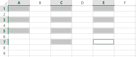
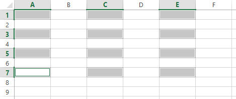
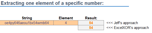
In that incarnation, you can use it to extract just one element of a specific number:
 

 
 

Or if you prefer, you can use this version:
=MID($A28,SMALL(IF(ISERROR(-MID(TEXT(MID(“||”&$A28,ROW(OFFSET($A$1,,,LEN($A28))),2),”|”),2,1)),FALSE,ROW(OFFSET($A$1,,,LEN
($A28)))),COLUMNS($B28:B28))-1,SUM(SMALL(IF(ISERROR(-MID(TEXT(MID(“|”&$A28&”|”,ROW(OFFSET($A$1,,,LEN($A28)+1)),2),”|”),{1,2},1)),
FALSE,ROW(OFFSET($A$1,,,LEN($A28)+1))),{1,2}+(COLUMNS($B28:B28)-1)*2)*{-1,1}))

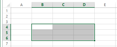
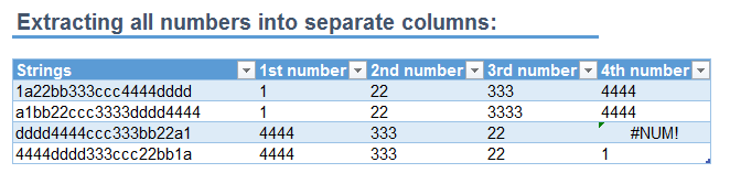
…you can use it to extract numbers into separate columns, where $A28 holds the string to be split, and B28 holds the first column that you want to extract a number to. Like so:
 

 
 

I don’t know how either of these perform against a UDF, let alone each other. Anyone got a lean, mean, UDF-based splitting machine that we can test it against?

Here’s a sample file:
ExtractNumber_20141120

—Edit 21 Nov 2014—
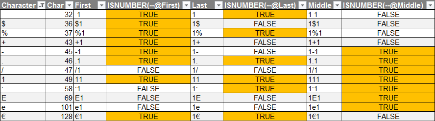
It turns out that my above formula fails for a few specific special character & number combinations. Here’s a table, showing in which cases Excel will still treat a number as a number when you pad it out with a non number. For completeness I do three tests:

• Special character before the number
• Special character after the number
• Special character on either side of the number

 

—Edit 8 Dec 2014—
Crikey…after chaining myself to the computer since the last update, I finally managed to cobble together a formula that will extract all numbers in practically any shape or form that the local version of Excel deems as a number. That is, given a string like this:
Jeff Weir Age: 43 DOB: 25/4/71 Salary: $100,000 StartTime: 8:30
…It returns this
43
25/4/71
100000
8:30

It ain’t pretty. If you like UDFs, then you’ll agree with my pal Gareth Hayter that this is pure formulabation. Unless you like formulas, in which case it’s orgasmic. (You sick, sick analyst, you. Don’t let your boss catch you playing with it in the office…)


=MID( String,SMALL( IF( ( FREQUENCY( ISNUMBER( -MID( String,ROW( OFFSET( $A$1,,,LEN( String)))*COLUMN( OFFSET( $A$1,,,,LEN( String)))^0,COLUMN( OFFSET( $A$1,,,,LEN( String)))*ROW( OFFSET( $A$1,,,LEN( String)))^0))*( COLUMN( OFFSET( $A$1,,,,LEN( String)))+ROW( OFFSET( $A$1,,,LEN( String)))-1),ROW( OFFSET( $A$1,,,LEN( String)+1))-1)=1)*ISNUMBER( -MID( "|"&String&"|",ROW( OFFSET( $A$1,,,LEN( String)+2)),1))=1,ROW( OFFSET( $A$1,,,LEN( String)+2))-1,FALSE),ROW( OFFSET( $A$1,,,LEN( String)))),SMALL( IF( ( FREQUENCY( ISNUMBER( -MID( String&"|",ROW( OFFSET( $A$1,,,LEN( String)))*COLUMN( OFFSET( $A$1,,,,LEN( String)))^0,COLUMN( OFFSET( $A$1,,,,LEN( String)))*ROW( OFFSET( $A$1,,,LEN( String)))^0))*( LEN( String)+1-ROW( OFFSET( $A$1,,,LEN( String)))),MOD( LEN( String)+2-ROW( OFFSET( $A$1,,,LEN( String)+1)),LEN( String)+1))=1)*ISNUMBER( -MID( "|"&String,ROW( OFFSET( $A$1,,,LEN( String)+2)),1))=1,ROW( OFFSET( $A$1,,,LEN( String)+2))-1,FALSE),ROW( OFFSET( $A$1,,,LEN( String))))-SMALL( IF( ( FREQUENCY( ISNUMBER( -MID( String,ROW( OFFSET( $A$1,,,LEN( String)))*COLUMN( OFFSET( $A$1,,,,LEN( String)))^0,COLUMN( OFFSET( $A$1,,,,LEN( String)))*ROW( OFFSET( $A$1,,,LEN( String)))^0))*( COLUMN( OFFSET( $A$1,,,,LEN( String)))+ROW( OFFSET( $A$1,,,LEN( String)))-1),ROW( OFFSET( $A$1,,,LEN( String)+1))-1)=1)*ISNUMBER( -MID( "|"&String&"|",ROW( OFFSET( $A$1,,,LEN( String)+2)),1))=1,ROW( OFFSET( $A$1,,,LEN( String)+2))-1,FALSE),ROW( OFFSET( $A$1,,,LEN( String))))+1)


Here’ a file showing how this bit of formulabation comes together: Dynamic Split Numbers_20141208 v6

Everybody knows that you can’t do some things with the result of an INDEX function unless you return it to the worksheet first. For instance, I can return the 2nd and 3rd members of the array {10,20,30} to the worksheet with an array-entered INDEX function like this:
 

 
 
…but if I wrap a SUM around that INDEX and array enter it, I get the wrong answer:
 

 
 
…meaning I have to return that INDEX function to the grid and then point my SUM function at it:
 

 
 
Everybody knows that, right? Well, everybody’s wrong. Everybody but the author over at the new ExcelXOR blog, that is. At this earth-shattering post the Author shows several intriguing ways to get INDEX to play nicely with outer functions:
 

 
 

Far out! That’s the kind of trick I would have sold my soul to the devil to learn.

There’s a lot to learn at that site: go to http://excelxor.com/blog/ and scroll most of the way down until the Archives section, and then get clicking. The earliest post is practically from yesterday: August 2014. But there’s a lifetime of learnings there already…both in the posts, and in the comments. Plus the most wicked formula challenges you will find in one place.

Sumit Bansal’s post VLOOKUP Vs. INDEX/MATCH – The Debate Ends Here! sparked some great discussion on the merits of VLOOKUP vs INDEX/MATCH, including at Oz du Soleil’s lighthearted rebuttal at The Anti-VLOOKUP Crowd Is Out In The Streets Again!

I especially love Peter B’s comment at Sumit’ post:

My opinion is that VLOOKUP and HLOOKUP are simply over-specialised legacy functions and Excel would be all the better for ‘pruning’ them out. I do use VLOOKUP occasionally when I have a 2-D range; the search array happens to be on the left; I only wish to return a single field; I am sure the data is clean and the match will always succeed. Despite that, I think the value they bring to the bloated zoo of Excel functions is not worth their keep.

Of course, NOTHING can ever be cleaned out of Excel, for good reason…otherwise all the millions of complex black-box spreadsheets that continue to function just fine long after the person who constructed them moved on to another task, job, or incarnation will break. Not to mention all those fantasy football spreadsheets. MS has backwards-compatibility issues that are beyond belief really.

At the same time I agree with Bob Phillips’ point at Sumit’s post:

The biggest selling point to me is that VLOOKUP is easy to teach to people, and it sticks, INDEX/MATCH less so.

But I disagree with Bob’s point that VLOOKUP can be/is just as flexible as INDEX/MATCH, merely because we can do stuff like this with it:
=VLOOKUP(“z”,CHOOSE({1,2},$B$1:$B$10,$A$1:$A$10),2,FALSE)
=VLOOKUP(“g”,$D$2:$H$15,MATCH(“Qtr2”,$D$2:$H$2,0),FALSE)

Just as flexible? Maybe, if you bend it double with brute force. Just as fast after you’ve made it just as flexible? Not likely. Any more understandable than the INDEX/MATCH equivalent? Not in my experience.

In fact, I feel a rude joke coming on:

Young analyst with unlit cigarette in mouth, having just consummated his first VLOOKUP: Has anyone got a match?
Analyst of distinguished years: Yes. Your VLOOKUP and my arse.

If MS were designing Excel from scratch – and I was on the committee that was deciding whether to include a dumbed-down function to do a subset of lookups based on hard-coded input parameters and a fixed data layout – then I’d make a case for not including it. Not just because of those quite reasonable complaints, either. But also because of evolution. A user that is forced to learn INDEX and MATCH due to lack of suitable alternatives is be better placed to evolve into a higher Excel lifeform than one that hasn’t looked beyond VLOOKUP.

(I’d make an exception if a major competitor – say Lotus – had a VLOOKUP function in their beast. But only in that specific case.)

Formulas remind me a bit like DNA: just by stringing a few different base-pairs together in the right order, you can build a mouse. Or a Human, with a few extra tweaks. Similarly, with a few good formula combinations under your belt, you can conquer most problems you’re likely to come across. INDEX and MATCH are not just formulas in their own right, but are the formula equivalent of DNA basepairs: they give users a peek into other formula ecosystems that they can gradually spread into and colonize. VLOOKUP ain’t one of those base pairs. It’s Neanderthal.

Hey, don’t get me wrong: I’m fine that it’s in the fossil record. I’m happy enough to have one in my spreadsheet, just as I’m happy enough to have an appendix that doesn’t burst.

…everyone complains about it, but nobody does anything about it. Well, certainly not Microsoft, anyhows. But back in 2012 Nigel Heffernan at Excellerando.Blogspot.com did: he put up some nifty code for joining and splitting two dimensional arrays that I just stumbled across. I thought I’d have a go at turning the join one into a function that can be called from the worksheet, and add a few more options while I’m at it. More butchering than tweaking, as you’re about to see.

My revision can be called from the worksheet, and has the following arguments:
=JoinText(Array,[Delimiter],[FieldDelimiter],[EndDelimiter],[SkipBlanks],[Transpose])

Yes, more arguments than at my last social outing. Most are optional and have defaults. Take that how you will. The default delimiter is a comma. The Field Delimiter is a separate Delimiter that gets added if your input array is 2D, and the default is also a comma. EndDelimiter puts an extra Delimiter of your choice on the end if you want one. Aesthetics only, really. The rest are explained below.

First, the result:

• That orange block is my data.
• Column D shows the result if you point the function at each respective row
• Row 8 shows the result of pointing the function at each respective column
• In rows 12 to 15 you see the result of pointing it at the entire 2D block of data, under different settings.

Those last two results are what happens if the data is laid out by row and then by column, and you’ve incorrectly told the UDF to transpose the input array. If your data happenned to be laid out like this, you wouldn’t need that Transpose argument:
 

 
 

The DelimitEnd argument does something pretty minor, really. If we include it, the end of the string gets padded with it – in this case an Exclamation Mark . If we exclude it, the string doesn’t get padded with any extra delimiters:
 

 
 

You might notice it skips blanks. It doesn’t have to, if you don’t want it to:
 

 
 

And it doesn’t need your two arrays to be the same size:
 

 
 

A real-world example where this might be useful is when concatenating lists of names, where some may have more parts than others:
 

Both the last two screenshots show examples of using three different delimiters…a space between words, a comma between columns, and something different on the end.

Here’s the code and workbook:
Join Function_20141115

Public Function JoinText(target As Range, _
Optional Delimiter As String = “,”, _
Optional FieldDelimiter As String = “,”, _
Optional EndDelimiter As String = “”, _
Optional SkipBlanks As Boolean = False, _
Optional Transpose As Boolean = False) As String

‘Based on code from Nigel Heffernan at Excellerando.Blogspot.com
‘http://excellerando.blogspot.co.nz/2012/08/join-and-split-functions-for-2.html

‘ Join up a 2-dimensional array into a string.

‘ ####################
‘ # Revision history #
‘ ####################

‘ Date (YYYYMMDD) Revised by: Changes:
‘ 20141114 Jeff Weir Turned into worksheet function, added FinalDelimiter and Transpose options
‘ 20141115 Jeff Weir Changed FinalDelimiter to EndDelimiter that accepts string, with default of “”

Dim InputArray As Variant
Dim i As Long
Dim j As Long
Dim k As Long
Dim lngNext As Long
Dim i_lBound As Long
Dim i_uBound As Long
Dim j_lBound As Long
Dim j_uBound As Long
Dim arrTemp1() As String
Dim arrTemp2() As String

If target.Rows.Count = 1 Then
If target.Columns.Count = 1 Then
GoTo errhandler ‘Target is a single cell
Else
‘ Selection is a Row Vector
InputArray = Application.Transpose(target)
Transpose = True
End If
Else
If target.Columns.Count = 1 Then
‘ Selection is a Column Vecton
InputArray = target
Else:
‘Selection is 2D range. Transpose it if that’s what the user has asked for
If Transpose Then
InputArray = Application.Transpose(target)
Transpose = True
Else: InputArray = target
End If
End If
End If

i_lBound = LBound(InputArray, 1)
i_uBound = UBound(InputArray, 1)
j_lBound = LBound(InputArray, 2)
j_uBound = UBound(InputArray, 2)

ReDim arrTemp1(j_lBound To j_uBound)
ReDim arrTemp2(i_lBound To i_uBound)

lngNext = 1
For i = j_lBound To j_uBound
On Error Resume Next
If SkipBlanks Then
If Transpose Then
ReDim arrTemp2(i_lBound To WorksheetFunction.CountA(target.Rows(i)))
Else
ReDim arrTemp2(i_lBound To WorksheetFunction.CountA(target.Columns(i)))
End If
End If
If Err.Number = 0 Then
k = 1
For j = i_lBound To i_uBound
If SkipBlanks Then
If InputArray(j, i) <> “” Then
arrTemp2(k) = InputArray(j, i)
k = k + 1
End If
Else
arrTemp2(j) = InputArray(j, i)
End If
Next j
arrTemp1(lngNext) = Join(arrTemp2, Delimiter)
lngNext = lngNext + 1
Else:
Err.Clear
End If
Next i

If SkipBlanks Then ReDim Preserve arrTemp1(1 To lngNext – 1)
If lngNext > 2 Then
JoinText = Join(arrTemp1, FieldDelimiter)
Else: JoinText = arrTemp1(1)
End If
If JoinText <> “” Then JoinText = JoinText & EndDelimiter

errhandler:
End Function


I like this function. I’m sure I’ll like it even more when you’re all finished polishing it to a bright sheen.

I like Doug Glancy’s UndoSelections code via his Selectracker utility. It allows you to deselect a cell from a selection that you made while holding the Ctrl Key…something that Excel doesn’t let you do out of the box. Nifty.

(Aside: If you’re NOT a Ctrl freak, then you can also put Excel into Add To Selection mode by pushing Shift + F8, which adds any further cells you click on to the current selection without the need to hold down Ctrl. When you’ve got the cells you want, just push Shift + F8 again.)

I thought I’d try a simpler approach…if the user tries to select something that’s already selected, simply dump it from the current selection. So I came up with this:


Private Sub Workbook_Open()
Set App = Application
End Sub

Private Sub App_SheetSelectionChange(ByVal Sh As Object, ByVal Target As Range)
Deselect Target
End Sub

Sub Deselect(Target As Range)
Dim lngCount As Long
Dim lngLast As Long
Dim strTarget As String
Dim strOld As String
Dim strNew As String

'This code allows you to deselect cells when CTRL + Clicking
strTarget = Target.Address
lngCount = UBound(Split(strTarget, ","))
If lngCount > 0 Then
strNew = "," & Split(strTarget, ",")(lngCount) & ","
'Need to add the "," as a delimiter so we don't incorrectly identify say $A$1 and $A$10 as the same
strOld = "," & Left(strTarget, Len(strTarget) - Len(strNew) + 1) & ","
If InStr(strOld, strNew) > 0 Then
If strOld <> strNew Then
strOld = Replace(strOld, strNew, ",")
End If
If Right(strOld, 1) = "," Then strOld = Left(strOld, Len(strOld) - 1)
If Left(strOld, 1) = "," Then strOld = Mid(strOld, 2, Len(strOld))
Application.EnableEvents = False
Range(strOld).Select
Range(Split(strOld, ",")(UBound(Split(strOld, ",")))).Activate
Application.EnableEvents = True
End If
End If
End Sub


Here’s an illustration: below is a screenshot where I was trying to select cells in a Checker-board pattern while holding Ctrl, but made a stuff-up a couple of clicks ago:
 

 
 

Without VBA, I’d need to start from scratch, because Excel doesn’t let you deselect particular blocks from your current selection. But with my trusty code, all I need to do is try to select the offending block again, and Excel will say Hey…you’ve already got that in your selection. Oh wait…I guess you’re trying to tell me that you want to dump that particular range from the selection, given it’s already selected.

And so it does just that:
 

 
 
…which frees me up to try again:
 

 
 
In fact, as long as I keep holding Ctrl down, I can deselect as many ranges as I want:

It works pretty well. See for yourself: Open the below sample file, hold Ctrl down and do some crazy clicking, and occasionally click something you’ve already selected. ZAP! It’s removed from the current selection.
Unselect_20141111 v3 (Note: I’ve updated this file with snb’s version of the code listed further below.)

Why this isn’t the native behavior right out of the box is beyond me.

There’s bound to be coding improvements, so let’s have ’em.

—UPDATE—

snb has a much smarter approach in the comments that lets users deselect individual cells within a particular subs-selection OR deselect a sub-selection in its entirety. I’ve amended the sample file accordingly.

His approach goes a little something like so:

Private WithEvents App As Application
Option Explicit

Private Sub Workbook_Open()
Set App = Application
End Sub

Private Sub App_SheetSelectionChange(ByVal Sh As Object, ByVal Target As Range)
Deselect Target
End Sub

Sub Deselect(Target As Range)

Dim rn As Range
Dim cl As Range
Dim sel As Range
On Error Resume Next
Set rn = Target.Areas(Target.Areas.Count)

If Target.Count > 1 And Target.Areas.Count > 1 Then
If Not Intersect(Range(Replace(Target.Address & "~", "," & rn.Address & "~", "")), rn) Is Nothing Then
For Each cl In Target
If Intersect(cl, rn) Is Nothing Then Set sel = Union(sel, cl)
If Err.Number <> 0 Then Set sel = cl
Err.Clear
Next
sel.Select
End If
End If
End Sub


And so with SNB’s code, if I were to select a block:
 

 
 
…and I wanted to ditch the cell in the middle, then I can simply select it while holding Ctrl, and it gets ditched:
 

 
 
Meaning that I can then say apply formatting, to create an in-cell donut:
 

 
 
Much better than my approach. Cheers, snb!

Well here’s something that I probably learned once, but have subsequently forgotten and then rediscovered: You can filter a PivotTable Page Field just by typing the PivotItem that you want to filter it on. So if I start with a PivotTable like this:
 

 
 
And say I don’t like the look of the mysterious substance that the kids have left smeared all over the mouse (probably just jam, but who the hell knows). I desperately want to filter that PivotField, but I desperately want to avoid the mouse. Well, watch what happens if I ust overtype the (All) in the PageField with the thing I want to filter by:
 
 
BING!
 

 
 
What’s more, if I type the name of a field that’s not already in the PivotTable over the existing PageField name:
 

 
 
…then Excel does something else intelligent: it says “Oh, you want me to bring that PageField into the Pivottable for you.”
 

 
 
The same thing in terms of adding new Fields goes for RowFields:
 

 

 
 
If you think about it, the adding of the fields is the same behavior as simply overtyping fields already in the PivotTable to rearrange them.

Regardless, now that this secret’s out, I don’t have to chip the sticky crap from my Mouse. As Phyllis Diller once said…Housework can’t kill you, but why take a chance? No, I don’t know who she is, either.

So if you’ve played around with Tables a fair bit, then you probably would have noticed that you can merrily insert a row in the worksheet that intersects one table:
 

 
 

…but if you try the same thing on a row that intersects more than one table, the Insert, Delete, and Clear Contents options are grayed out (or greyed out, if you live where I live):
 

 
 

You may have tried to get around Excel’s veto by cutting or copying a row from somewhere else, then trying to insert it via the ungrayed (or ungreyed) Insert Copied Cells option:
 

 
 
…at which point Excel wiped that smirk of your face with this:
 

 
 

So I know when this happens. But I don’t understand why. Anyone have any ideas?

I’ve been playing around with the Formula Auditing tools a fair bit recently. These things:
 

 
In the course of this, I noticed a few things I haven’t before. Firstly, here’s my setup:
 

 
 
When I have cell D6 selected and click Trace Precedents, Excel is kind enough to draw just one arrow from the precedent range, while putting a box around the entire Precedent range so I can see where it is:
 

 
 
If I were to click on Trace Dependents for that cell, I’d like to see pretty much the same thing:
 

 
 
…but here’s what I actually see:
 

 
 
…which looks like something that Hippies were hanging on the walls in the late sixties:
 

 
 
…when they weren’t out protesting, that is:
 

 
 
Doing a Trace Precedents when there’s a much longer array of dependent cells involved looks even worse:
 

 
 
…and Excel becomes very sluggish as you scroll around, so presumably Excel is constantly redrawing these. Scrolling down doesn’t tell you much…that’s for sure:
 

 
 
Let’s take a look at another setup, to better illustrate a couple of things I didn’t know until now:
 

 
 
Here’s what Trace Dependents has to say about cell B2:
 

 
 
One thing I didn’t realise until today, is that if you keep clicking that Trace Dependent button, Excel keeps drawing in additional levels of downstream dependents:
 

 
 


 
 
In case you didn’t know, you can double-click on any of the blue arrows, and you’ll be taken to the Precedent/Dependent cell concerned…particularly handy if it points somewhere off-screen. And you can double-click the arrow once you’re there to be magically transported back again. The dotted arrow pointing to a little sheet icon in the above screenshot tells you that there’s an off-sheet dependent that points at cell C19, which you can jump to if you double click on that dotted arrow and then select the reference from the Go To box:
 

 
…although as you see above, the native dialog box is so narrow that you’re unable to actually see the cell addresses, and can’t be resized. In that case, you might want to download Jan Karel’s excellent RefTreeAnalyser, that fixes this and does a good deal more besides:

 
It also has a much better way of displaying precedents, by overlaying in the current window some little pictures of any precendents that happen to be out of view or on another sheet. (Would be really handy to have the same functionality for dependents too.):
 

 
 
Colin Legg has some great code that will also help you to determine all on-sheet and off-sheet precedent cells, using the .NavigateArrow method to actually travel up those blue arrows and thus find any precedents on other sheets. I imagine Jan Karel uses pretty much the same approach. [Edit: No, he doesn’t ]. You’ve got to use the .NavigateArrow method, because the Range.Precedents property doesn’t return precedents on other sheets or other workbooks.

Now here’s something nasty I’ve just noticed about the native Formula Auditing tool: It doesn’t pick up on off-sheet references that involve any kind of Table Reference, although on-sheet references work just fine:
 

 
 
So it is well broken, in my opinion, because I often refer to Tables on other sheets. And both Colin’s code and Jan Karel’s addin won’t help you here, I’m afraid. [Edit: Jan Karel’s code still catches these.] Seems to me the only way to get around this would be to search the worksheet for instances of a Table’s name occurring within formulas. That’s assuming there’s no way to actually read Excel’s dependency tree from wherever Excel maintains it. I seem to recall seeing a post a few years back about how you can extract information from the tree by extracting XML from the workbook file, but that might just be a flight of fancy. Anyone know whether it ispossible to interrogate the dependency tree directly somehow?

How ’bout colours instead of Arrows?

Given all those arrows can get pretty confusing, I thought I’d have a crack at coding up something that lets you use Conditional Formatting instead and/or arrows to highlight Dependents (Green) and Precedents (Blue). Here’s my starter for ten, with both Dependents and Precedents highlighted. Direct Dependents/Precedents get a darker colour and white bolded font so you can easily tell them from indirect:
 

 
…and you can restrict it to just showing direct:

 
…and overlay arrows if you want:
 

 
 
It automatically updates if you change your selection, too:
 

It doesn’t solve the Table issue mentioned above, but I’ve been finding it quite handy to get a quick feel for what’s going on in those crappy spreadsheets I inherited…err…designed recently.

Here’s a sample file:
FormulaAuditing_20141112