A couple of days ago I floated the concept of a dedicated annual “Still Broken” week in which we can talk very honestly about the things in this otherwise great application that we think are still broken, plus review our list from the same time last year to see if any action has been taken by our gracious host…that would be Microsoft…to actually remedy anything we were bitching about the previous year. And just as importantly, to give credit where credit is due…because let’s face it…it’s not trivial to make changes to something that 750 million odd users are using at the time.
100% of the comments of that post that directly mentioned this concept were generally supportive (thanks, Doug). So I thought “There’s no week like the present”.
And so, without further ado, here’s a bit of Excel that I was playing with today that strikes me as being not quite finished: the Add-ins options.
Why is it that if I save a brand new Add-in to the Add-ins folder:
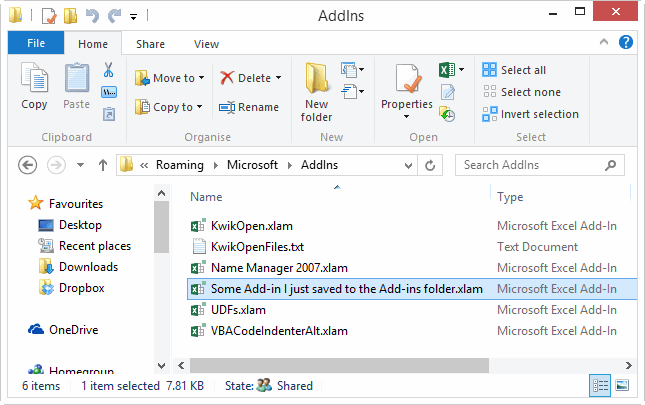
…it doesn’t automatically show up in this window, under the Inactive Application Add-ins section?
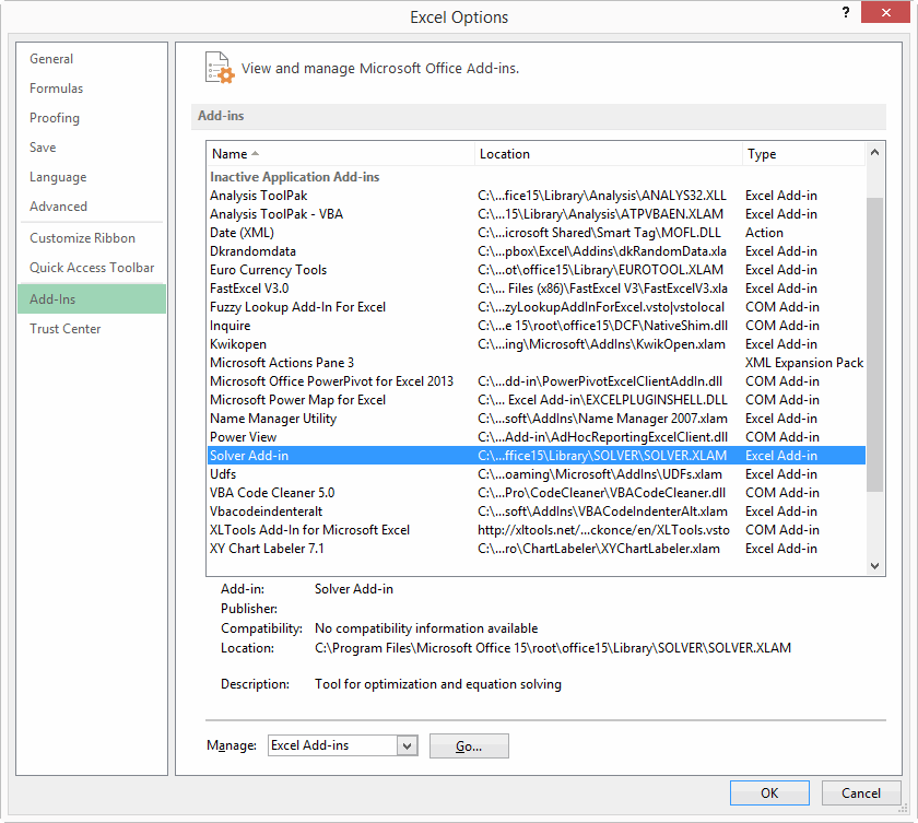
…and yet if I click the Go button next to Manage Excel Add-ins, I see that Excel obviously knows about it: Edit: And even though I parked it in the right car-park building, it still won’t show up until I politely point Excel to the exact spot I parked it in:

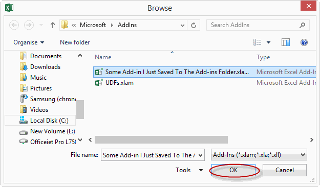
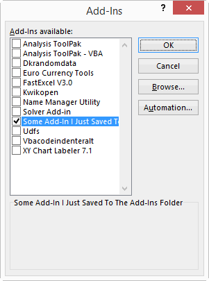
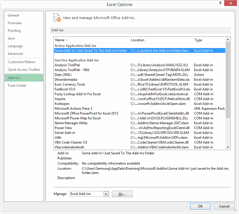
Given it was correctly stored in the Add-ins folder, why didn’t you just let me automatically populate it into the ‘Inactive Application Add-ins’ part of the Excel Options/Add-ins pane like this from the get go:
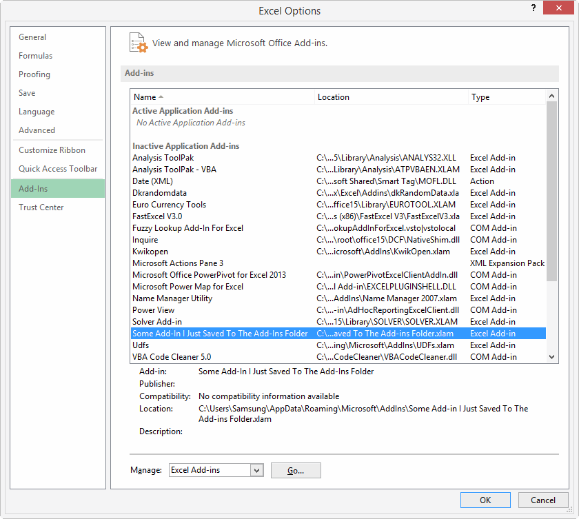
…and then let me decide to activate it just by double clicking on that listing?
Currently, selecting an Add-in from that Excel Options dialog and double clicking does absolutely nothing. What’s the point in letting me even select it…it’s not like I can actually do anything with it. All you’re doing is giving me vain hope.
Furthermore, jumping back a few steps now, whenever I push OK from that Add-ins dialog box:
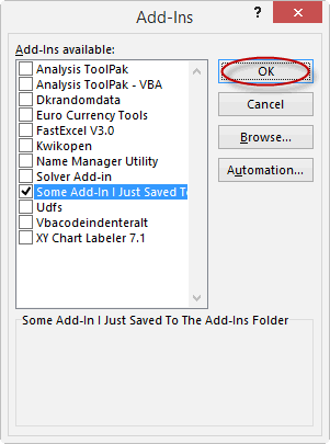
…why do you automatically assume I’m done with the Excel Options dialog box I came from, and close it? Is it inconceivable that I might want to manage more than one Add-in? Or that my intention was to manage a COM add-in, but I forgot to change that default Excel Add-ins option in the dropdown, and want some simple way to go back and choose the other option? Sheesh.
Please Microsoft…don’t make me click. Here’s a thought: hire someone to the newly created position of “Manager, Click Reduction”, and empower them to champion basic design changes that let users use your interface much more efficiently. I’m available.
In fact, I think you need to take an honest look at what you expect users to do in order for them to leverage off of Add-ins. I think the current system presents too much of a barrier to non-technical people who would otherwise be able to make much more out of your fine application. I’ve just spent quite a few days writing the chapter in my book that explains how users can leverage off of Add-ins without having to have one jolt of knowledge of VBA. Unfortunately, my conclusion is that while they don’t have to be VBA experts, they do have to be “Install an Add-in” experts, because the process is not as simple and genius as it could be.
Okay, that’s kick-started the week. Who’s up next. Anyone? Anyone?
I can’t play this game, because although there are many things in Excel 2010 that I think are unfinished (or even broken since Excel 2003 and in need of repair), I don’t know which of them have already been fixed in Excel 2013.
I would like to set the standard format for dates. We use “d mmm yy” for short and “ddd, d mmmm yyyy” for long format. No dashes, no back slashes, and only one comma after the week day. It is very annoying that we have to go in and format the cells every time we create a date.
Derek…just assume none of them have. We’ll let you know in the rare case that they have.
@Kevin: Just go into control panel, region and language and adjust your date format there. That is what Excel uses.
To all: 80 percent of all feature requests Micrsosoft gets for Excel are already in the product :-)
My wishes…
Make all dialogs sizable. And I mean ALL. So this includes the F5 (Goto) box.
Forms Design : Why has this not improved in 20 years? (I don’t have a copy of 2013, so please correct me if I am uninformed)
‘Ghost Projects’: when you close a workbook, the VBA project remains visible in Project Explorer.
This induces errors if you’re repeatedly opening and closing files during testing: it’s too easy to waste time editing and testing code in a ‘Ghost Project’, only to lose it all when you try to save and close.
Like Derek, I’m on 2010, but here’s my biggest annoyance: I have a table named tblTest (columns = Name and Number) and I have a formula in a cell
. I position my cursor just after the equal sign and type
and press Tab to complete the ‘Number’ column reference. The result is
. The MATCH function name is erased.
If I type a space, then arrow back and type the INDEX function thereby leaving a space between what I’m typing and MATCH, it still erases MATCH (and the space). If I type a period, then arrow back and type the INDEX function, it still erases MATCH (and the period).
The only way to prevent it that I’ve found is to type the entire column name and not press Tab to complete it.
The Add-Ins dialog and presumably the Options dialog only show the contents of the Add-Ins library at the time that Excel was opened.
I hate the announcement asking if you want to replace the file that was already there. It seems to have nothing to do with an add-in, and what it asks isn’t what it means.
Where to start? When I save a chart type as a template I get a Windows folder to work with, but when I want to use the template I get a bunch of uninformative icons. I can mouse over them to see their names, but I can’t sort them in any other order than name order. So I end up naming a lot of templates with multiple underscores (more underscores than the last time I did that).
There is a “Manage Templates…” button, but that doesn’t let me select the template I want.
Also, the templates ought to reliably work on the data, tested by applying the saved template to the very chart you saved the template from. Frequently they fail to reproduce the original chart.
Hi Derek.
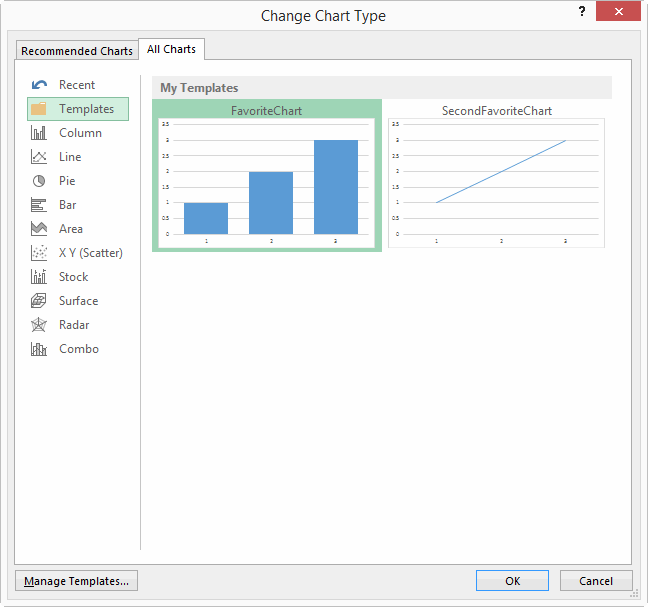
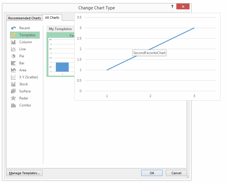
I assume you’re on Excel 2010 or earlier? From memory, that used to annoy the hell out of me too.Yes, you are using Excel 2010. You’ll be happy to note that things are improved in Excel 2013. Here’s how templates look in 2013:…and if you hover over them, the preview gets bigger:
Better?
Granted, you need to stump up the upgrade fee if you’re not on Office 365 package. (And let’s face it, if you ARE on the Office 365 package then you have stumped up the upgrade fee, effectively).
But let’s give credit where credit is due:

Thank you, the Microsoft Charts Team. We appreciate your improvement. Well done. Print this off and stick it on the cubicle wall:
@Jan Karel: I’d add “And while you’re at it, make the ones that do resize open to a more generous size from the get go. Can’t you work out how big my monitor is, and resize accordingly?” .
I hate it how I constantly have to manually resize windows that are about as generous in their native proportions as a hobbit. Gentlemen prefer elves, thank you very much.

@Randy, you’re not uninformed. Forms are as beautiful now as they were then.
@Nigel, I very rarely get that. Does it happen often?
@Dick, yeah, you’ve mentioned that one before at http://dailydoseofexcel.com/archives/2014/01/24/yes-please-vs-wtf/#comment-122831 , and this one bugs the heck out of me too. But as Sam says over at that post, They fixed this problem in the Measures Window of Power Pivot, so if you say =Calculate(Sa and Tab it will complete Sales with a Close Square bracket. It should just take 3 or 4 more versions before they fix it in Excel’s Table References
@Jon, yeah I noticed that one as well. Another unwelcome example of click tax.
My unfavourite “feature” is discussed here:
https://newtonexcelbach.wordpress.com/2012/09/05/when-is-an-xy-chart-not-an-xy-chart/
In fact there are two features that badly need fixing here (make that three if you include the Microsoft insistence on referring to XY graphs as scatter charts).
On an XY chart you can plot a large number of separate lines as a single series by simply leaving a blank cell between each line, which is good.
If you enter a space (or any other text) in one of the blank cells Excel decides that you really need to have a Line chart instead of an XY chart, or maybe they decide to make your XY chart look like a line chart. Either way, there is no way of switching this behaviour off, which is bad.
But what makes it really bad is that if you are generating your data as a VBA variant array, there is no way to return truly blank cells to the worksheet. Either you get a value of 0, or you get a cell that is treated as text.
It would be good if this could be fixed before next Mar 14, but that’s probably expecting too much. I just hope it’s fixed by Mar 14, 2115.
Another ‘Not quite finished’ feature: changing the scope of a named range.
We do now have a dialog for editing a name, but the ‘Scope’ dropdown is disabled. So the only way to reduce the scope of a workbook-level name to a sheet appears to be deleting the name and redefining it.
Yes, there are excellent third-party add-ins for this: but those add-ins exist because of a limited OEM interface.
Non-resizable File Explorer dialogs…
Seriously, who decided that you’d only ever want to view six files at a time in the Explorer dialogs for selecting reference dll’s, button images, and any ‘insert file’ action?
Doug, when i tried Empty within a vba array it didn’t appear on the XY plot – maybe this is fixed in 2013 version or maybe i am doing something different. Otherwise can you not use CvErr(xlErrNA) instead?
On a related note, one thing that bugs me is inconsistent treatment of ranges and arrays. Why are arrays allowed as chart series and defined names but not in most other things (validation lists, database criteria, sparklines, pivot tables, …)? It would be nice to be able to have this data off the sheet.
And yes to comments about sizeable dialogs, the formula evaluation window is another that would really benefit.
Nigel: Yes, there are excellent third-party add-ins for this: but those add-ins exist because of a limited OEM interface.
You nailed it. As per my rant in the previous post, that’s actually a key point of the book I’m writing – Excel for Superheroes and Evil Geniuses. The Evil Genius is someone who has a powerful arsenal of ‘borrowed’ technology at their disposal in the form of some killer User Interface tweaks, User Defined Functions, and weapons-grade Add-ins that they use to pimp Excel so that it runs faster, meaner, and leaner than even a Superhero could make it run.
Of course, the Evil Geniuses of my book only need code because the Excel UI holds even Superheros back due to some poor choices in UI design. Your point of course is that they shouldn’t have to become Evil Geniuses just to fix suboptimal stuff that has no right being broke in the first place.
Oh, and I just got me one of those ghost projects in the VBE. Spooky.
My least favorite dialog box is the Text Import Wizard
Five rows!
Lori – I just checked with 2013, the problem only occurs with a UDF, from a Sub vbNullString and Empty both return a blank cell, which leaves the XY chart displaying properly. This is the same as in previous versions.
Using CvErr(xlErrNA) in a UDF keeps the XY chart display as XY, but then the two nodes either side of the #NA are connected, whereas the point of the blank row is to plot the lines as two separate segments.
New Dot Functions Have Limited Functionality
You still can’t use the new statistical functions in Named Formula that reference Named Ranges as the x Values
There is a bug in the implementation of the new .DIST Functions in Excel 2010 & 13
If I setup two Named Formula
Y: =NORMDIST(x,mean,sd,FALSE)
X: =Row(Offset(Sheet1!$A$1,,,40,1))
where:
x is a named formula of values between 0 and 20 in steps of 1.0
mean = 10
sd = 2.5
I can Plot Y vs X and get a nice Bell shaped curve.
Save the file
=============
If I now change the Named Formula function to
Y: =NORM.DIST(x,mean,sd,FALSE)
Excel crashes as soon as the Enter is pressed or the Tick is pressed in the Named Formula Dialog to accept the formula
I have tried the above concept on all the Statistical functions and the same error applies to all the new .DIST functions
I use Excel 2010 + 13 (64 bit) and Windows 7.
Space and period didn’t fix my annoyance, but an open parenthesis does.
Then edit and inlude an open paren
Then you have to left arrow to get to the left side of the paren. Start typing the outer INDEX formula
When you get to the second argument, delete the inserted paren, go to the end of the formula and continue the typing.
Yes, the cure is almost worse than the disease.
@doug, right there’s a user setting for plotting empty cells as gaps so for consistency i think a similar option should be added for other non-numeric values. A workaround is to right-click individual points after blanks and select to remove connecting lines or else write a udf to do this (since udfs can modify charts) but it’s not ideal.
All the PLY menu items (right-click a sheet tab) should be available via the ribbon. Also we should be able to unhide more than one sheet at a time.
Excel and Xml are a great couple, ever since 2003. However, there is a need for a few “improvements”:
– Excel should allow the export of empty tables without alert;
– when importing empty tables Excel should delete ALL listrows under ALL conditions (bug);
– when importing empty tables Excel should preserve the columnformulas and -formatting (bug).
See for details: http://pixcels.nl/xml-observations/
The Excel object I use most is the listobject (after the range naturally). It is so annoying that the listcolumn doesn’t have a property ColumnFormula (string, read/write).
How about this one? The Autofilter object has three filter types: text, number and date. They are superb, use them every day. But why does the Filter object doesn’t have a Type property? There is no way we can determine from vba which filter type Excel is showing in the userinterface, besides inspecting the column content.
Lori – I didn’t know it was a setting, it’s always worked that way for me.
” A workaround is to right-click individual points after blanks and select to remove connecting lines or else write a udf to do this (since udfs can modify charts) but it’s not ideal”
Especially if you have a series with 10,000 line segments :)
The previous comment reminds me of a couple of serious performance issues that have been around since I started using Excel.
Creating a drawing with a lot of lines (about 1000 or more) is very slow. The drawing creation time seems to be about proportional to the number of lines squared (i.e. 10 times as many lines takes 100 times as long, rather than 10 times as long). There has been some improvement in 2010/2013, but its still very slow.
Transfer of large arrays between the spreadsheet and VBA is very slow. In some recent tests I found a speed difference of nearly 500,000 times on performing some simple data extraction from large arrays.
https://newtonexcelbach.wordpress.com/2015/02/20/slicing-arrays-with-vba/
Some loss of performance is inevitable, but a factor of 500,000 is just ridiculous.
Frans: great suggestions. I hope someone is getting this stuff down.
So here’s another example of the Add-Ins option not being quite finished.
You delete an Add-In from the Add-Ins folder using Windows Explorer. Next time you open Excel, you see this:

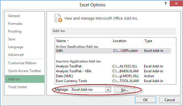
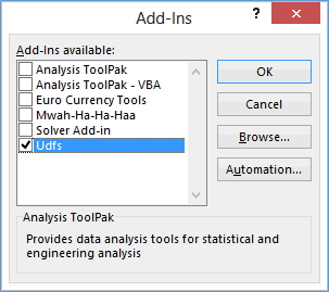

But are you given an opportunity to actually do anything about it? Nope. They make you go into “Manage Addins” before you can fix it:
And finally you get the opportunity to do something about it after unchecking this:
…at which point this comes up:
So why didn’t you just give me that option initially?
By the way, anyone notice my brilliantly named Add-In in that Add-Ins Available list?

It’s from my new book. I just love opening Excel now, and seeing this:
Wham, bam, thank you .xlam!
My pal Gareth suggested an even better addin name:
“Opening: porn websites, sending screenshots to all of your contacts.xlam (100%)
I’ll have another go: I produce a lot of charts of time series, and if I want them to not be hideous I often have to resort to non-pivotChart charts, and helper columns in the table instead of transformed date formats in the Pivot.
There should be more flexibility over the display of dates in Pivot Tables, when the dates have been Grouped. In 2010, once you group dates, they display as mmm-yy with a hyphen, and you can’t have any other format.
There should be better multi-level category axis displays in Pivot Charts, when the horizontal axis is grouped dates. If I want years, then months as single letters, or week-endings, then days of the week, that should be possible.
If I want one level of multi-level category axis labels to be aligned horizontally, and another to be aligned vertically, according to the space available, that should be doable.
Excel displays calendar months of the year as single letters, but doesn’t do that for days of the week. There should be a “ddddd” format that displays the week as “M”, “T”, “W”, etc. (I’m aware I can create a TEXT formula in the source table to achieve this)
[yes there’s the potential for confusion between Tuesday and Thursday, or Saturday and Sunday, but that’s not a problem when displaying the series on a chart. Anyway you could say the same about the single letter months]
@Jeff
That addin name is as bad as my “Federal Police Surveillance Van” WiFi network name
@Frans
In addition to your XML suggestions:
In some XML structures, Excel refuses to repeat the value of parent items in the table do you end up with rows which have a blank “parent” column. Not so great of you want to do Pivottables for instance.
@Hui: Absolute gold. But you can do better: “ISIS recruitment team” should scare the natives.
Other stuff?
The HelpFile and HelpContextID parameters for message boxes and inputboxes (and raised errors) are now broken: you can’t pass the ‘Help’ button parameters of an existing Office help topic.
The MS Forms DataObject is still firmly stuck in the 20th Century; and with it, our programmatic access to the clipboard. Unless you’re willing to take on a very complex API calls.
Determining the dimensions of an array still requires deliberately raising an error, or a CopyMem API call.
There’s no ‘PasswordChars’ option for textboxes and input boxes. So any interaction that requires a password from the user (other than the native UI for opening password-protected workbooks) involves typing out the password en clair.
…Typing out passwords in plain text on-screen is really, really bad security (and it breaks legally-mandated accessibility guidelines for everyone using a screen reader). However, the API code to poke asterisk chars into an Input Box dialog is quite chewy.
That’ll do for now. And, gosh, it’s not all bad news: we no longer need an API call to widen the ‘Name’ box!
Also @Hui and @Jeff: “Surveillance_Vehicle_4” has been my WiFi router name for a while now, give or take rotating the number every couple of days. On April Fool’s day, I got it to display the equivalent PinYin characters: please don’t to this from your RV’s WiFi router if you’re visiting the Claude Moore Colonial Farm in Virginia, or driving through the Southern suburbs of Cheltenham Spa.
@headtoadie – Yes, unhide more than one sheet at a time!
I love the tables feature, especially how formulas can refer to field/column names rather than cells. But after seven years of copying the formulas from on table column to another, I wish I could set absolute and relative references to the field names. If I copy the cell, all internal (to the table) references are treated as absolute. But if I drag the cell, then all internal references are treated as relative. I wish I could control that. When I am working with a table that is doing some summary by month, I’m glad there are only 12 months in a year.
Omar: there is a workaround for this. See http://www.excelcampus.com/tips/absolute-formula-references-excel-structured-table/ and also check out Jon’s free addin while you’re there.
Hi Jeff. Thank you for the pointer. I’ve studied the solution and think I understand it. I even have the add-in installed; just annoying that it always opens up two screens over from my work screen (but then, so does the Find/Replace window)!
I might have a case that breaks that tip, though. Take this formula:
=SUM([@M3]:[@Mcurrent]
I want it to adjust to
=SUM([@M4]:[@Mcurrent]
In my little bit of testing, I can’t seem to make that happen in a way that I can drag. Oh well. I already have this particular report working, and I don’t see doing any quite like this again (I hope).
Thanks again. The link was very helpful.
@Nigel: I assume you are not referring to textboxes on userforms, which do have a PasswordChar property?
biggest pain – lack of a negative lookup column on vlookups to go to the left of the index field. Lotus used to have it. Match+Index is an “alright” workaround, but a negative direction column would be easier.
I am by far not as advanced as many but I feel like ranges should have the option to automatically expand when the range is named. In example if I set up a range, I could be able to put a checkmark by rows and any rows added to the immediate bottom of that be incorporated into the range. I know there are many workarounds but it seems like it is over complicated.
Thanks so much!
Indeed the addin manager is a dreadful contraption, a historical accident! It was a while ago but as it was unfriendly I made my own addin manager.
Briefly, it displays a list of all loaded addins and a second list of available but unloaded addins, maintained in a main list (a text file) of all addins previously added to it (via a button click), or found in one of the default addin locations, and/or in the addins collection. From the ribbon one click to display the lists then double click to load or unload a selected addin from either listing. It’s simple to use but there’s quite a lot of housekeeping involved and it took a long time tweaking until it worked as I wanted. I work a lot with addins but it’s very rare I ever look at the builtin manager!
In the Format Cells===Numbers====to be able to format cells as Feet and Inches such as 1´ 8″ or 1´/8″ or 1´-8″
Missing from above comment is fractions of an inch such as 1/4, 1/8, 13/16, 31/64 etc.
Peter, that sounds great. I’d be interested in taking a look sometime, if you’re open to sharing.
thanks for sharing !
@Jeff: Sure, I sent an email to your “info” address yesterday, if you didn’t get it…
@Jeff,
As much as I appreciate the ISIS suggestion, I like the suburb/house I live in
I am sure Jail doesn’t have the same feel
Nor would a big smoking hole in the ground, once the drone strikes.
@Alicia: Excel Tables (introduced in Execl 2007) are effectively just that: automatically expanding names that Excel maintains on your behalf.
@Jan Karel – Textboxes on UserForms do indeed have a PasswordChars property – but not on worksheets.
There’s a limit to how secure password input can be in Excel and VBA, but ‘best practice’ in most applications is to pass it straight from a transient input dialog to the consumer object, without using explicit variables – they are more persistent than you think – and persistent textbox objects.
It’s not the fear of unauthorised access via an illegal (but unnoticed) memory access – Excel and VBA are vulnerable to far simpler attacks than that! – it’s a pragmatic admission that every identifiable operation my code performs on a password is a possible error.
My suggestion: an Excel option to set Ctrl+V to paste values by default. I’ve requested this twice.
I know there is the AppKey+V trick, but this is something the product should have.
MS forgot to adapt the VBA function ‘Index’ to the resized worksheet (rows.count & columns.count) in Excel 2007.
So in VBA the 2003 rows.count is still the limit in 2015, resulting in:
working correctly:
erroring out:
Any time a third party utility add-in is popular, it’s a sign the original app wasn’t properly finished. I mentioned the lack of chart labeling before, that XL13 has finally dealt with. Have they made Jan Karel Pieterse’s Name Manager redundant yet? I just ran into the problem that in Excel 2010:
1) Define Names chooses “Workbook” scope by default
2) You can’t alter the scope once you’ve chosen it
3) You can’t Apply Names using names with Workbook scope, even in the same worksheet as the named ranges
These three phenomena together mean either persuading colleagues at work to get JKP’s product, or telling them they’ve got to do it all the hard way.
(I had what I thought was a great sequence of keyboard actions to quickly create and apply a bunch of range names without hassle, but the above shortcomings mean it doesn’t work)