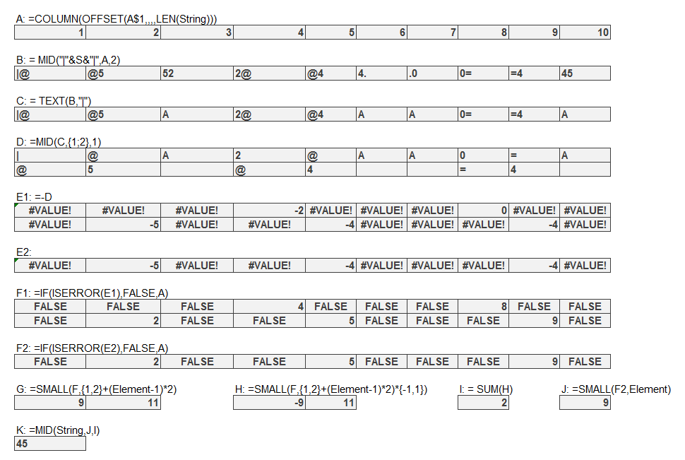
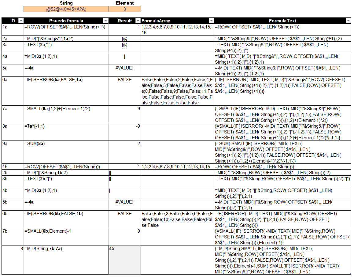
Since Excel 2013, Microsoft has given us a FORMULATEXT function, which if you point at a cell will do just that. Here’s a naughty snapshot of FORMULATEXT playing with itself in the corner:

I thought I’d have a go at writing a FormulaArray function to complement it, because when I’m building up a complicated formula that uses lots of array manipulation, then I like to document how all the different arrays within it fit together. (I was going to say “come together” there, but after that crack about FORMULATEXT playing with itself, I thought better of it. But now that I’ve said crack, I’m gonna throw caution to the wind and say wind too.)
Currently I document my formula beasts by either either array-enter a sub-part in the sheet with some notes, like this:

…which shows how my ExtractNumber formula works, or I enter the desired formula in one cell with a ShowFormula to the left and a hand-rolled hard-coded array to the right, like in this table where I’m documenting a few ways to dynamically generate consecutive integers:

I get that ResultArray manually, by clicking in the formula bar, pushing F9, copying the resulting evaluated array, then pasting it in another cell. Tedious. Especially when I later make a change to that sub-part, because then I get to do those steps all over.
So I started to roll my own FormulaArray function. I got a bit bogged down in the joining bit, but after about an hour of Googling, I rediscovered Nigel Heffernan’s code for joining two dimensional arrays. Which is very concerning, because I discovered it like just 10 days ago, and even wrote an extensive blog post on it right here. Senility is obviously setting in. If I start saying the same thing over and over like my mother does, just shoot me. If I start saying the same thing over and over like my mother does, just shoot me.
Anyways, Nigel’s function needs a 2D array. You can create an array from formula text by using VBA’s Evaluate method. If the formula returns a Row vector or a 2D vector, then Evaluate nicely turns it into a 2D vector. But here’s the rub: if the formula returns a Column vector, then Evaluate only gives us a 1D vector, which ain’t gonna wash with Nigel’s function:

So what we need to do is TRANSPOSE any formulas that would return Column vectors, because chucking a TRANSPOSE into the mix has the desired effect:

Note that I’m using the square brackets [ ] shortcut for Evaluate. I could just have easily done it like this:

Okay, so we know that if our formula string returns a Column vector, we’ve got to transpose it. But how can we tell that ahead of time? I can’t think of a way. So I just do this:
Function FormulaArray(Target As Range) As String

Dim strInput As String

Dim var2 As Variant

Dim lb As Long
strInput = Mid$(Target.Formula, 2)
var2 = ActiveSheet.Evaluate(strInput)
On Error Resume Next
lb = LBound(var2, 2)
If Err.Number <> 0 Then
var2 = Application.Transpose(ActiveSheet.Evaluate(strInput))
FormulaArray = Join2d(var2, ",", ";")
Else:
FormulaArray = Join2d(var2, ";", ",")
End If
End Function
So I evaluate the formula as if it’s a Row vector, then check if I’ve got 2 dimensions as a result. If not, it must have been a column vector, in which case I transpose it, then reevaluate it. Shame about the double evaluation, but I can’t think of a foolproof way to do it differenty, other than perhaps array entering the formula into a 2D range on the worksheet and looking at where the #N/A! errors fall.
Anyway, it seems to work just fine:

..unless you happen to be using Structured Table References, and your arguments happen to use the @ table notation to point at something on the same row:

…or unless you happen to have a formula with the INDIRECT function in it:

With the ThisTableRow thing, I guess I can just replace the @[SomeColumn] bit with the actual address, but I can’t think of easy ways around the INDIRECT thing. Anyone got any ideas?
Edit: Thinking about this some more, all I need to do is substitute the INDIRECT(SomeExpression) with whatever gets returned by RANGE(SomeExpression).value
Sample workbook:
There’s a handy post over at Charles Williams’ site that talks about some other quirks of Evaluate that’s worth checking out:
https://fastexcel.wordpress.com/2011/11/02/evaluate-functions-and-formulas-fun-how-to-make-excels-evaluate-method-twice-as-fast/
You might as wel look at
http://www.snb-vba.eu/VBA_Fill_combobox_listbox_en.html#L_0
How to fill a combobox/listbox using the method ‘Evaluate’
Wouldn’t this be sufficient for your formulaarray ?
Function F_snb(c00 As Range)On Error Resume Next
F_snb = Join(Evaluate(Mid(c00.Formula, 2)), ";")
If Err.Number <> 0 Then F_snb = Join(Application.Transpose(Evaluate(Mid(c00.Formula, 2))), ";")
End Function
@snb:
Thanks for the link to your site. I’ve never seen it and it has tons of great stuff!
You really need to find a topic for the letter Z. It looks lonely.
Hi snb. Testing the result of the Join is a good idea, but your approach doesn’t handle 2D arrays, such as =ROW(INDEX($A:$A,D2):INDEX($A:$A,E2))*{1,2}
I see from that that I don’t need the final argument of the MID function, so there’s an efficiency saving. I think I prefer the approach of using var1 to hold the formula string, in case I need to evaluate it again…although I realize now that I needn’t use a Variant to do that, so have changed it to a string. And I should use Mid$ instead of MID. Not that I’ll ever notice the performance gains from these deckchair rearrangements.
maybe try this code in a new module which works around some vba Evaluate limitations. eg:
B2
=TRANSPOSE(ROW(INDIRECT(“1:4”))+{0,4})
B3
=EvalCell(B2,1)
[={1,2,3,4;5,6,7,8}]
B4:E5
=EvalCell(B2)
[with CSE]
Private Sht As Worksheet Const Tmp = "__Tmp" Function EvalCell(Target As Range, Optional Formula = False) Set Sht = Target.Worksheet Dim AddTmp: AddTmp = "'" & ThisWorkbook.Name & "'!AddTmp" Run AddTmp & "(" & Target.Address(External:=True) & ")" Run AddTmp & "(" & Mid(Sht.Names(Tmp).Value, 2) & ")" If Formula Then EvalCell = Sht.Names(Tmp).Value Else EvalCell = Sht.Evaluate(Tmp) Run AddTmp & "(NA())" End Function Function AddTmp(V) If IsObject(V) Then V = Application.ConvertFormula(V(1).Formula, xlA1, xlA1, True) Sht.Names.Add Tmp, V, False End Function (Note: may need modifications for structured references.)@Mike
Thank you.
I will add ‘Zen and the art of VBA maintenance’
@Jeff
You are right but I only wanted to show that testing isn’t necessary:
Function F_snb(c00 As Range) as stringOn Error Resume Next
F_snb = Join(Evaluate(Mid(c00.Formula, 2)), ";")
If Err.Number <> 0 Then
err.clear
F_snb = Join(Application.Transpose(Evaluate(Mid(c00.Formula, 2))), ";")
end if
if err.number<>0 then F_snb=Join2d(var2, ",", ";")
End Function
When writing UDFs one thing that should strictly be done but is generally neglected is to refer references relative to an appropriate cell (usually either Application.ThisCell or a reference argument.) This is because a reference like “C4” in a formula or a range argument could change value depending on which sheet is active when the formula is calculated.
To see this enter a formula in cell B2 of a blank sheet then in another cell enter: =FormulaArray(OFFSET(B2,,1)). Now type something on a new sheet and the result of the formula will change. This is due to use of Application.Evaluate or ActiveSheet.Evaluate, instead you can use: Target.Worksheet.Evaluate. Similarly in the function i posted, the line:
Run AddTmp & "(" & Mid(Sht.Names(Tmp).Value, 2) & ")"should be updated to include a workbook reference. One possible replacement would be:
Run AddTmp & "(if({1}," & Split(Target.Address(External:=True), "!")(0) & "!" & Tmp & "))"Lori: your approach of writing the formula as a Named Range and then reading the RefersTo range is very, very, very clever.
Re your second comment, =FormulaArray(OFFSET(B2,,1)) returns nothing for me in both cases. What am I missing?
@jeff: apologies, it should be OFFSET(B2,,). The suggested change was to allow the formula to reference other sheets eg with Sheet2!B2 as the argument.
And thanks, it’s not really that clever though. It uses the feature that Application.Run evaluates the first argument internally which allows you to some things like define temporary names that you can’t do normally (since it is effectively run on a separate thread.) On a side note, the functions IFERROR and IFNA appear to do something like this by creating a temporary name that can be seen in the names collection with a _xlfn. prefix.
@Lori,
In general IMHO, UDFs should never contain any hardcoded (cell) references. Anything the UDF needs from Excel should be passed as arguments. That avoids ambiguity.
@jkp: agree that any range references should be made explicit in arguments which also ensures dependencies are properly defined for recalculations. When passing strings containing cell or named references they also need qualification to avoid ambiguity, for example:
Function Eval(Formula)
    Application.ThisCell.Worksheet.Evaluate(Formula)
End Function
But in practice the reference to the calling cell is usually omitted here (eg http://superuser.com/questions/253353/excel-function-that-evaluates-a-string-as-if-it-were-a-formula) which can lead to incorrect evaluations when the function is calculated with another sheet active. This frequently happens when formulas contain volatile functions.
oops, was too quick in posting should be:
@Lori: I tried your approach on the various components of my ExtractNumber formula, and it doesn’t return an array for any of the below where the outer formula is MID or TEXT. I haven’t looked into why yet.
—EDIT— Nor does my approach either. Weird.

Jeff, did you try with the revised line i suggested? snb makes the point that you can place an “INDEX(…,)” around the formula to force array evaluation. i think “IF({1},..)” works for this as well.
Hi Lori.Yeah, yours failed too. I put a screenshot in the comments of the previous post that illustrates this. I’ll try the IF({1} and see what happens.
Whoops, I thought this comment was at the other post. No, I realise now I haven’t tried with your revision. Will take a look.
@Lori: Weird…I ran your code the other day, and it worked just fine. But today, your code doesn’t seem to return an array for me at all, but only the first item in the array – no matter whether I’m using the original line or the amended line – and it seems to run very very slowly. Tried it on two different files on two different PCs.
My bad…forgot the optional argument of 1.
@Lori: What IS weird is that having a RUN command in a UDF makes that UDF volatile, and there doesn’t appear to be any way around it. To see what I mean, put Debug.Print “Volatile” somewhere in your function, and any time you make a change anywhere in the sheet, you’ll see that printed twice to the immediate window.
This is giving me the correct results:
Function F_snb(c00 As Range) As StringOn Error Resume Next
F_snb = Join(Evaluate(Mid(c00.Formula, 2)), ";")
If Err.Number <> 0 Then
Err.Clear
F_snb = Join(Evaluate("transpose(" & Mid(c00.Formula, 2) & ")"), ";")
End If
If Err.Number <> 0 Then
For Each it In Evaluate("index(" & Mid(c00.Formula, 2) & ",)")
c01 = c01 & ";" & it
Next
F_snb = c01
End If
End Function
@jeff: i hadn’t noticed that – interesting find! Adding a statement at the end of the function stops the volatility for me, as in the below example:
Function test()
    Run "abc()"
    Application.Volatile False
End Function

Function abc()
End Function
I suppose it’s a good idea for a UDF to be volatile when evaluating a random string so it might be intentional to mark the cell as dirty with a run statement. Having said that if you change the line to: Run “abc” (without the parentheses), it now isn’t volatile and you can step through it – but you can’t then use this in a UDF to add a name. So it is definitely quirky!
Reminds me of something weird that came up in the last excelxor challenge where SUMIF automatically expands the last argument eg =SUMIF(A1:B1,1,C1) but this is volatile?! One way to see this is to append: +abc(), and add a break point to the function.
Btw, have been enjoying your recent witty and insightful series of posts – this one a little close to the line perhaps :)