Getting data from an Excel sheet into an array is usually best accomplished with a statement that looks something like this:
|
1 |
vMyArray = Sheet1.UsedRange.Value |
I thought it would be keen to fill an array from a filtered list, so I coded
|
1 2 3 4 5 6 7 8 9 |
Sub ArrFilteredList() Dim vArr As Variant vArr = Sheet1.UsedRange.SpecialCells(xlCellTypeVisible).Value Stop End Sub |
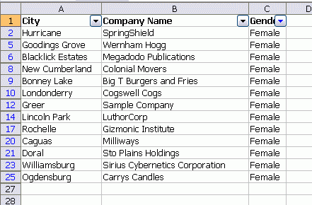
on this list

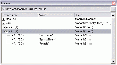
The SpecialCells returns a range of only those cells that are visible, i.e. unfiltered in this case. The problem, it turns out, is that this method doesn’t work with noncontiguous ranges and that’s just what SpecialCells returns. I put the Stop in there so I could check the Locals Window.

It filled from the first Area of the range, then stopped. I confirmed that it was the lack of continuity of the range with this code:
|
1 2 3 4 5 6 7 8 9 |
Sub ArrNonContiguous() Dim vArr As Variant vArr = Union(Sheet1.Range("A1:C1"), Sheet1.Range("A4:C6")).Value Stop End Sub |
which returned similar results. So I’m stuck iterating through the range, I guess. But then my array is backward; column, row instead row, column because I can’t change the first element of an array with Redim Preserve.
|
1 2 3 4 5 6 7 8 9 10 11 12 13 14 15 16 17 18 19 20 21 22 23 24 |
Sub ArrFilteredList2() Dim rRow As Range Dim aArr() As String Dim i As Long Dim lCount As Long ReDim aArr(1 To 3, 1 To Sheet1.UsedRange.Rows.Count) lCount = 0 For Each rRow In Sheet1.UsedRange.Rows If rRow.Hidden = False Then lCount = lCount + 1 For i = 1 To 3 aArr(i, lCount) = rRow.Cells(i).Value Next i End If Next rRow ReDim Preserve aArr(1 To 3, 1 To lCount) Stop End Sub |
Is there a better way?
‘Uses a variant array
‘Uses the range that is auto filtered
‘Transposes the filled array
‘Me thinks you may have something else in mind?
Sub ArrFilteredList2()
Dim rRow As Range
Dim vArr As Variant
Dim i As Long
Dim lCount As Long
Dim af As AutoFilter
Dim rng As Range
Set af = ActiveSheet.AutoFilter
Set rng = af.Range
Set rng = rng.Offset(1, 0).Resize(rng.Rows.Count – 1, rng.Columns.Count)
ReDim vArr(1 To 3, 1 To rng.Rows.Count)
For Each rRow In rng.Rows
If rRow.Hidden = False Then
lCount = lCount + 1
For i = 1 To 3
vArr(i, lCount) = rRow.Cells(i).Value
Next i
End If
Next rRow
ReDim Preserve vArr(1 To 3, 1 To lCount)
vArr = Application.Transpose(vArr)
‘Stop
MsgBox UBound(vArr, 1) & vbCr & UBound(vArr, 2)
End Sub
Are you committed to using an autofilter? If not, an advanced filter extracting to a new range would do the trick. Or, a SQL query perhaps?
The simplest way:
copy the cells to an empty space
read the data there
.autofilter 1,“test”
.offset(1).copy sheets(1).cells(1,27)
.autofilter
End with
sq=sheets(1).cells(1,27).currentregion
sheets(1).cells(1,27).currentregion.clearcontents
I forgot
.autofilter 1,“test”
.offset(1).specialcells(xlcelltypevisible).copy sheets(1).cells(1,27)
.autofilter
End with
sq=sheets(1).cells(1,27).currentregion
sheets(1).cells(1,27).currentregion.clearcontents
I might be tempted to read the full (unfiltered) range into an array (to keep the number of sheet read actions down) and then put each row into a collection element, filtering out unwanted elements during the process.
I tend to do my manipulations on the collection elements, then write to an array to load onto the sheet, but you could load the array from the collection before manipulation.
I DO like geoff’s SQL idea, though.
This worked for me…
“”‘
Dim rRow As Range
Dim aArr() As Variant
Dim i As Long
Dim lCount As Long
Dim CellCount As Variant
Dim Range_To_Get As Variant
CellCount = Sheets(1).UsedRange.Rows.Count
Range_To_Get = Sheets(1).UsedRange.Address
ReDim aArr(1 To 3, 1 To CellCount)
lCount = 1
i = 1
For Each rRow In Sheets(1).Range(Range_To_Get)
If lCount = 4 Then
i = i + 1
lCount = 1
End If
If rRow.Rows.Hidden = False Then
aArr(lCount, i) = rRow
Else
GoTo Devo:
End If
lCount = lCount + 1
Devo:
Next
ReDim Preserve aArr(1 To 3, 1 To i)
aArr = Application.Transpose(aArr)
End Sub
Good Luck
Devo
If AutoFiltering is enabled, and an AutoFilter is in effect, AutoFilter.Range appears to be a pseudo UsedRange which includes all cells in scope for auto-filtering. The range it refers to doesn’t change with different filtered row counts.
I used Intersect, feeding in xlVisible and AutoFilter.Range to get what I needed to create a chart from the filtered rows.
(You have to adjust AutoFilter.Range to remove the first row).
Not thoroughly tested as I’m referring back to an old bit of code.
Any good?
I think that the problem with your original approach to handling a filtered list, is that the range returned by Sheet1.UsedRange.SpecialCells(xlCellTypeVisible) within the line
vArr = Sheet1.UsedRange.SpecialCells(xlCellTypeVisible).Valueis a range containing multiple "areas" or non-contiguous parts. So we should be able to process each area, which is a contiguous range, individually. However, the approach of just assigning everything into "vArr" will not work, because one can not control the part of vArr which should be filled by the next assignment. The copy function, as suggested by Hans, is able to handle multiple areas within a range, as is demonstrated when you copy from filtered rows or cells, and paste into some empty worksheet. I suspect the easiest to code method is as Hans suggests above, using an intermediate empty space. If no empty space for holding the intermediate result is readily available, then I think the most direct method would be something like what you ended up with, after a few changes, as follows:
Sub ArrFilteredList2()Dim rRow As Range, aArr() As String, i As Long, lCount As Long, CurrRng As Range
ReDim aArr(1 To 3, 1 To Sheet1.UsedRange.Rows.Count)
lCount = 0
For Each CurrRng In Sheet1.UsedRange.SpecialCells(xlCellTypeVisible).Areas
For Each rRow In CurrRng.Rows
lCount = lCount + 1
For i = 1 To 3
aArr(i, lCount) = rRow.Cells(i).Value
Next i
Next rRow
Next CurrRng
ReDim Preserve aArr(1 To 3, 1 To lCount)
Stop
End Sub
In addition, it would be possible to repeat the loop to count the number of rows in each of the areas, in order to know the correct dimensions for aArr before it is redimensioned the first time. That information would allow the rows and columns to be reversed by removing the need for a redimension with preserve, with corresponding changes in the value assignment statement of course. That may be closer to what you really wanted, and would look like:
Sub ArrFilteredList2()Dim rRow As Range, aArr() As String, i As Long, lCount As Long, CurrRng As Range
lCount = 0
For Each CurrRng In Sheet1.UsedRange.SpecialCells(xlCellTypeVisible).Areas
lCount = lCount + CurrRng.Rows.Count
Next CurrRng
ReDim aArr(1 To lCount, 1 To 3)
lCount = 0
For Each CurrRng In Sheet1.UsedRange.SpecialCells(xlCellTypeVisible).Areas
For Each rRow In CurrRng.Rows
lCount = lCount + 1
For i = 1 To 3
aArr(lCount, i) = rRow.Cells(i).Value
Next i
Next rRow
Next CurrRng
Stop
End Sub
If the intent is to get a table’s filtered column for use in something like a Combobox, then I prefer this:
Function Filter2Array(oTable As ListObject, vColumn As Variant) As Variant' @BXL/CWH
Static oClipBoard As Object
Dim vArray As Variant
If oClipBoard Is Nothing Then Set oClipBoard = _
CreateObject("new:{1C3B4210-F441-11CE-B9EA-00AA006B1A69}")
oTable.ListColumns(vColumn).Range.SpecialCells(xlCellTypeVisible).Copy
oClipBoard.GetFromClipboard
vArray = Split(oClipBoard.GetText, vbCrLf)
ReDim Preserve vArray(LBound(vArray) To UBound(vArray) - 1)
Filter2Array = vArray
End Function
A hack would be to sort the list by the column you want to filter, then apply the filter. This would leave all visible cells contiguous.
What if you have filters on several columns?
And amount of data is really huge (full table is something like 30 columns and > 200,000 rows)?
@Craig Hatmaker
I know this is few years old…. But i have been using your clipboard method for ages.
It now fails with one of my users – no clear error, it just returns an empty array. If I debug I can see that there are cells getting selected.
Are there any common clipboard issues or reference problems?
hi
i found this way:
Sub …
Dim ArrCrit as variant
…
With Worksheets(“Sheet1”)
.ListObjects(“List1”).ShowAutoFilter = False
.ListObjects(“List1″).Range.AutoFilter Field:=2, Criteria1:=”+”
ArrCrit = GetVisibleRowsArray([List1].SpecialCells(xlCellTypeVisible))
End With
…
End sub
Function GetVisibleRowsArray(FirstArray As Range) As Variant
Dim iResRow&, iRow&, ArrLenght&
Dim iArea As Range
Dim ResultArr() As String
‘On Error Resume Next
ArrLenght = FirstArray.Count / 2
ReDim ResultArr(1 To ArrLenght, 1 To 2)
iResRow = 1
For Each iArea In FirstArray.Areas
For iRow = 1 To UBound(iArea.Value2)
ResultArr(iResRow, 1) = iArea.Value2(iRow, 1)
ResultArr(iResRow, 2) = iArea.Value2(iRow, 2)
iResRow = iResRow + 1
Next iRow
Next
GetVisibleRowsArray = ResultArr
End Function
I know that this is quite old, but I came across this situation myself recently and wanted to share how I went about it. I did cheat a bit, as I used a few of Chip Pearson’s Array functions (http://www.cpearson.com/excel/vbaarrays.htm): IsArrayAllocated, and CombineTwoDArrays (the latter relies on another of his array functions, NumberOfArrayDimensions). But I thought it worked out nicely:
Don’t care how old it was, that was very useful Russell. Thanks for posting that.