Spellchecking One Cell

When you apply the CheckSpelling method to a one-cell range, Excel continues to check the rest of the sheet and prompts you to continue spellchecking from the beginning of the sheet. You can use Application.DisplayAlerts = False to remove the prompt, but it still checks more than just that cell.

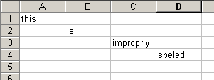
Excel range with two misspelled words

Sub CheckSpell()
    ‘Checking one cell will result in a prompt
   Range(“C3”).CheckSpelling
End Sub

message box to spellcheck from beginning

Tom Ogilvy noted in a recent newsgroup post that extending the range to more than one cell solves both problems.

Sub CheckNoMsg()
    ‘this eliminates the prompt, but still checks D4
   Application.DisplayAlerts = False
    Range(“C3”).CheckSpelling
    Application.DisplayAlerts = True
   
    ‘This checks c3 only – kind of
   Union(Range(“c3”), Range(“iv65536”)).CheckSpelling
End Sub

Combining, via Union, the range in question with a cell that we know to be empty (IV65536 in this case) limits the spellcheck to one cell – actually two, but who’s counting.

Changing the System Cursor

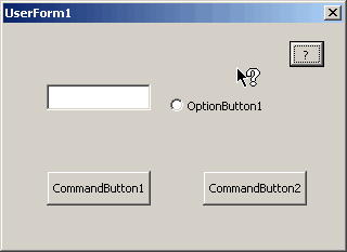
I was thinking about implementing a “What’s This?” type help system on an Excel userform. The first task, it seems, is changing the cursor. In Changing the Cursor in VBA, I discussed the built-in way to modify the cursor. The options there are pretty limited and they particularly don’t include a question mark that I might like to use for this application.

AllAPI.net had an example from Jerry Grant that seemed to fill the bill. It uses several API’s of which I understand most. I modified the example a little to suit the situation. Here is the declaration section of a standard module:

Option Explicit
 
Public Declare Function CopyIcon Lib “user32” _
   (ByVal hIcon As Long) As Long
 
Public Declare Function LoadCursorFromFile Lib “user32” Alias “LoadCursorFromFileA” _
    (ByVal lpFileName As String) As Long
 
Public Declare Function SetCursor Lib “user32” _
    (ByVal hCursor As Long) As Long
 
Public Declare Function SetSystemCursor Lib “user32” _
    (ByVal hcur As Long, ByVal id As Long) As Long
 
Public Declare Function GetCursor Lib “user32” () As Long
 
Public Const lOCR_NORMAL As Long = 32512

And here is the code behind the userform that changes the cursor.

Private mbWhatActive As Boolean
Private mlCurrCursor As Long
Private mlDefCursor As Long

Private Sub cmdWhat_Click()

    If mbWhatActive Then
        ChangeCursor
        mbWhatActive = False
    Else
        ChangeCursor “C:Windowscursorshelp_r.cur”
        mbWhatActive = True
    End If
   
End Sub

Private Sub ChangeCursor(Optional sCursPath As String)
   
    Dim lCursor As Long
   
    If Len(sCursPath) = 0 Then
        lCursor = mlDefCursor
    Else
        mlCurrCursor = GetCursor()
        mlDefCursor = CopyIcon(mlCurrCursor)
        lCursor = LoadCursorFromFile(sCursPath)
    End If
   
    SetSystemCursor lCursor, lOCR_NORMAL
   
End Sub

I was messing around with cursors, and I think I like this one the best:

userform showing changed cursor

Setting MultiSelect in Code

Jason points out a problem with setting the Multiselect property of a Listbox using VBA, as opposed to setting it manually at design time. Take this code:

Private Sub UserForm_Initialize()
 
    Dim sht As Worksheet
   
    Me.lstSheets.MultiSelect = 2
   
    For Each sht In ActiveWorkbook.Worksheets
       Me.lstSheets.AddItem sht.Name
    Next sht
 
End Sub

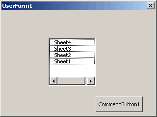
It produces this userform with unsightly rectangles around each list entry.

Listbox with rectangles around all entries

This happens with MultiSelect = 1 or 2, but not zero. If you must change this property in code (and Jason does, but I’ve simplified his situation for this example), do it after you populate the control.

Private Sub UserForm_Initialize()
 
    Dim sht As Worksheet
   
    For Each sht In ActiveWorkbook.Worksheets
       Me.lstSheets.AddItem sht.Name
    Next sht
   
    Me.lstSheets.MultiSelect = 2
   
End Sub

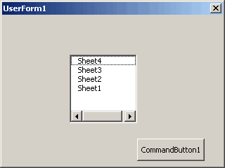
Listbox with rectangle around first entry only

Good question, Jason. I rarely set that property at run time, but if I do, I can’t have my Listboxes all rectangly.

A Rose by Any Other

Tuesday will be the one year anniversary of Daily Dose of Excel. Thanks to everyone for reading. It’s been a lot of fun, and educational, writing these posts. Thanks also to the other contributors for the excellent work they’ve done over the last several months. Finally, special thanks to JWalk for encouraging me to do this and helping me out in the early days.

I came up with the name “Daily Dose of Excel” in about 90 seconds, and I’ve hated it ever since. Well, ‘hated’ might be too strong. I’ve always wished I would have spent more time and had a cooler name. I’m considering changing the name and thought you might have a few ideas for me.

Since it’s been a year, it might be fun to have a contest. That will give me a chance to spend some of my hard earned Google revenue. The worst thing about a contest is writing the rules such that I don’t have to declare bankruptcy, so be sure to read the last one carefully.

  • Send me an email with your suggestion for a new name for this site. The current name will be considered in the voting, so don’t bother telling me you like the current name – it’s already in the running.
  • You must send the name via the link above or in such a way that I can’t tell that you didn’t.
  • You must send the email from the same email account with which you registered on this site. If you’re not registered, you can’t win. If you used a fake email to register, just include that fake email address in your message so I can confirm you’re registered.
  • The best three or four names will be listed with the current name and a vote will be taken. The name that gets the most votes wins.
  • I may not change the name, even if a different name wins. In other words, it’s totally up to me what I’m going to do. But there will still be a winner even if the name stays the same.
  • One submission per registered reader.
  • If two people send the same name, the first one received will get that name. If two names are similar, the one I use, if any, will be the one to get that name.
  • The winner will get to choose between a copy of Professional Excel Development or Excel VBA Programming for Dummies.
  • To be eligible, the entrant must live in a place that Amazon.com will ship to and where the shipping will be less than the cost of the book.
  • Any other rules that make this contest less of a burden on me or that I may choose to enact retroactively or otherwise

Okay, if I missed any rules or you need clarification, post a comment. Otherwise, start the hamsters and send an email. If I don’t get three suggestions, I’ll probably just buy myself a present. If I do get three, expect a poll early next week. I suppose I’ll need to find a way to vote that’s more secure than the polls I have been using.
TextColumn Property

I never noticed this Listbox property before, but it seems like it could be useful. According to help, the TextColumn property sets the column whose value the Text property will return. The BoundColumn property determines what the Value property returns, so this seems to bet the step sister of that.

You can now have easy access to two columns in a multicolumn Listbox. I don’t really see a downside since everything in a Listbox is text anyway, so the difference between Value and Text should be nothing. If you don’t set the TextColumn property, the Text property returns the same as Value.

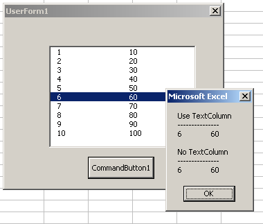
This example shows two ways to access a different column than the BoundColumn: One using the List property and one using the Text/TextColumn properties.

userform and message box showing results

Adding Comments II

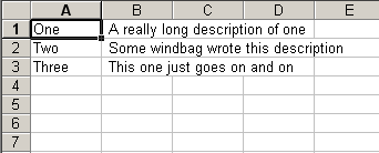
In Adding Comments, I read the data from a text file and created comments with one of the fields because it was large. I mentioned in that post that the way I wouldn’t do it is to import the text file normally, then a run macro. I don’t think it’s necessarily a bad way, it’s just not my preference.

I start by importing the text file using File > Open. That brings up the Import Text wizard and results in a sheet like this:

Text file after importing into Excel

In a separate file, I have a macro. The separate file could be an add-in, for instance, but it doesn’t have to be. The code just can’t be in a text file.

Sub MoveColumnToComment()
   
    Dim ws As Worksheet
    Dim rCell As Range
    Dim rRng As Range
   
    Set ws = ActiveSheet
    Set rRng = Intersect(ws.Columns(1), ws.UsedRange)
   
    For Each rCell In rRng.Cells
        rCell.AddComment rCell.Offset(0, 1).Value
    Next rCell
   
    ws.Columns(2).Delete
   
End Sub

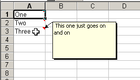
Once the code is run, I’m left with:

Excel range after macro showing comments added

Adding Noncontiguous Cells

I’ve found myself in the situation where no matter where I moved my cursor, the selection was extended. This is usually because I accidentally hit the F8 key to enter Extended Selection mode. I don’t think I’ve ever used it on purpose.

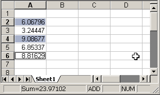
However, in my never-ending quest to rid myself of the mouse, I used a feature I’ve never used before: Shift-F8 to enter Add mode. I had a list of five numbers and I wanted to see the sum of the first, third, and fifth numbers. Normally, I would use the Control key and the mouse to select the three cells, then read the SUM in the status bar.

To do this with just the keyboard, I found the Add mode, but I still don’t think I’m using it right. To get the below SUM, I did the following:

  1. Start in A2
  2. Press Shift-F8
  3. Arrow down to A4
  4. Press Shift-F8 to exit Add mode
  5. Press Shift-F8 again to reenter Add mode
  6. Arrow down to A6
  7. Read the sum

Three noncontiguous cells selected

That double Shift-F8 key sequence can’t be the best way, but I’ll be damned if I could come up with a better one.