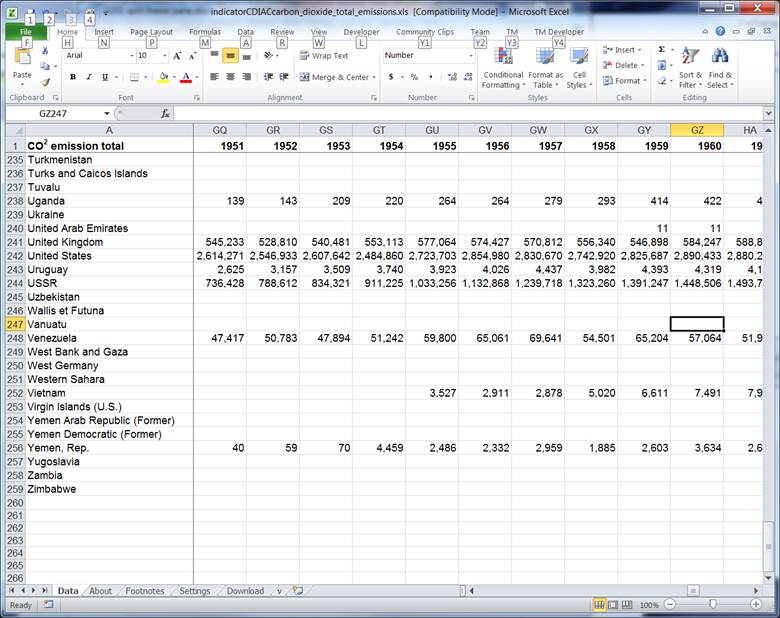
When working with a worksheet that contains a large number of rows and/or a large number of columns with row and column headers, it is very helpful to always view the headers no matter where one scrolls through the document.
An example is shown below. The table lists the year-by-year carbon dioxide emissions by country (the data set comes from data download page at Gapminder – http://www.gapminder.org/data/). The current worksheet view shows data from the 1950s (columns GQ through GZ) and countries that are alphabetically towards the end of the list of countries (rows 235 through 259). At the same time, the column headers (row 1) and the row headers (column A) are still visible. This lets one quickly establish a context for the numbers. This is the result of using Excel’s Freeze Panes feature.

A complementary feature is called Split Panes. The key differences between freeze pane and split pane are the somewhat different behavior while scrolling and an easier way to adjust the panes, which, of course, comes with extra responsibility to manage the risk of accidental changes to the split panes configuration.
For a version in a page by itself (i.e., not in a scrollable iframe as below) visit http://www.tushar-mehta.com/publish_train/xl_vba_cases/0201%20split%20freeze%20pane.shtml