I’m up to about March 15th in my backlog of emails. Tonight I read two emails about encryption: one from Wolfgang and one from Keith. I’m waiting to hear back from Wolfgang on what I think may be an interesting idea, but Kieth has a challenge that I know you’ll like. He explains it very well, so I’ll shut up and let him do the talking:

I have a 5 x 5 range that is empty, let’s say A1:E5
I also have a similar 5 x 5 range (assume G1:K5) with formulas in each cell
such that each cell displays a separate letter of the alphabet (skipping J),
as below:

A B C D E
F G H I K
L M N O P
Q R S T U
V W X Y Z

Now for the tough part… I want to be able to type letters into the first
range of cells (left to right, beginning on line one) and have those letters
displayed in the corresponding cells of the second range, HOWEVER!!!!, I
want the remaining letters of the alphabet to be displaced accordingly so
that no letter is repeated… here’s an example for the word “BARK”:

In the first range, I type:

B A R K

The second range displays:

B A R K C
D E F G H
I L M N O
P Q S T U
V W X Y Z

Notice that the letters for bark have simply been moved to the top row and
the remaining letters have been shuffled accordingly. All the remaining
letters of the alphabet remain in alphabetical order. Obviously, the user
would need to ignore repeated letters in his word, so the word CHEATERS
would be typed as:

C H E A T
R S

(Not typing the second E) and the result would be:

C H E A T
R S B D F
G I K L M
N O P Q U
V W X Y Z

For the life of me, I cannot figure out what formula(s) will give this
result in the second range of cells. In case you’re wondering, this little
matrix is used in the field of cryptology (enciphering and deciphering
messages). Specifically, the enciphering method that uses this matrix is
called the “Playfair” method (and also the “Double Playfair” method) and was
used by both the Axis and the Allies in WWII. Any solutions (or partial
solutions) you could provide would be greatly appreciated.

I have a solution that uses two helper ranges. I don’t know if helper ranges are allowed, though. I’ll post mine tomorrow.

Jim T. sends this along, and I’m not sure what’s causing this behavior. Maybe you know and comment on it.

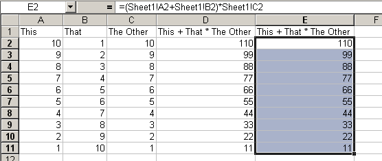
Col. D and Col. E are identical except that Col. E’s formula has range references that include the sheet name.

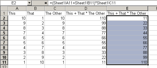
If you sort Col. D without sorting any other data on the sheet, you get the expected result (at least the result that I expect). That is, nothing happens. The formulas move to a different location and their range references change relatively. The formula that references A2, moves to D11 and then references A11. It looks like nothing happened.

Why then when I sort Col. E, does the same thing not happen? It sorts based on the values, but the formulas don’t change. Or maybe they do change – however you want to look at it.

I have a lot of good ideas. Particularly, ideas for applications for which I never seem to have the time or motivation to start, much less complete. My latest idea is a scoring system for my golf league. Last season I would get the weekly updates on an Excel spreadsheet and I would cringe in horror. No data integrity. No formulas beyond simple SUMs. I don’t expect the commissioner to be an Excel guru, so I don’t blame him. There’s just a better way. This year, I volunteered to keep score and made all kinds of promises about how great the scoring system would be. One of the promises was that it would be complete by noon today. That ain’t happenin’.

A couple of days ago, I start putting this app together. I start in Excel – it’s what I know and what I intended to use. In a short time, I abandoned Excel for Access. When I start thinking about applications, the first thing I think about is data stores. What is the nature of the data I need to store and where am I going to store it? Sixteen golfers times 15 weeks times nine holes is 2,160. Why would I incur the additional setup of an Access database when I could simply store it in a worksheet?

I set up worksheets for Teams, Players, Courses, Schedule, Weeks, and Scores. I then set about creating a userform to populate the Scores table, drawing data from the other tables to ease data entry. That’s when I say to myself “Self, this would be so much easier in Access because all the form-to-table code is built in”. It also seems to be easier to query the data in Access. I scrap the workbook and start setting up the mdb, importing all my “tables”, so I really don’t lose much time.

Everything’s going great. I’ve created some relationships and some queries to get some of the easier data out of tables. Then I hit a snag. I need to compute everyone’s handicap with our special handicap algorithm. It requires me to know the last three scores each golfer has posted. Easy enough except for the fact that not everyone plays every week. A golfer’s last three scores could be from weeks 5, 4, and 1 and another is from weeks 5, 4, and 3. I’m not strong enough in SQL to create this query. After an hour of banging my head on the desk, I decide that the best course is to write a UDF that determines the third most recent week a golfer has posted a score. I can then use that in my query and it will be peachy.

I get done with the first draft of this UDF and I have a thought. As long as I’m writing this 40 line UDF, why don’t I just make it a 60 line UDF and have it return the handicap. Just do all the work in the UDF. It works out most awesomely. Now that I know the handicaps, I can write a query to determine who is the A golfer and who is the B golfer (two man teams). Correction: Someone could write that query, but it’s not me. Back to the module to write another UDF to spit out the golfer I want.

I have this terrific set of tables, a beautiful relationship screen, and a couple of good queries. By the time I’m done writing my second UDF to compensate for my lack of SQL ability, I start asking myself why I’m doing this in Access. If I’m going to be doing everything in UDF’s anyway, I might as well go back to Excel where at least I can write code without consulting the help file every two minutes or trying to remember the proper syntax of a where clause.

Should I use Excel as a front end and Access as a data store? That’s a possibility, but I’m not sure what I’d be saving. Instead of creating queries via the Access UI, I’d be writing straight SQL in my VBA code. That doesn’t sound too attractive. Maybe I can have the best of both worlds, though. Maybe I can use ADO when it’s easier to do in a query and I can use CopyFromRecordset to a worksheet when it’s easier that way. Keeping the data in Access will also provide some scalability when, for instance, I want to php this to a website.

You know you’re a hack when you have two half-done apps in two different development environments and you still don’t know which one you should use.

Created by Laurent Longre:

The problem – how to create an array of filtered items in a column
list. The SUBTOTAL function allows you to operate on an array of this
type with a limited number of worksheet functions, but it does not
expose the array for formula manipulation. Laurent came up with an
elegant solution to this problem, based on an obscure behavior of
the OFFSET function. It turns out that when an array is used as the
2nd argument of OFFSET, such as

=OFFSET(Rge,ROW(Rge)-MIN(ROW(Rge)),,1)

an array of RANGES is returned. If the array is properly sized, as in
this example, the OFFSET function returns a separate single cell range
for each cell in the original range(Rge). Thus, if this array of arrays
is operated on by the SUBTOTAL function, each single cell range gets
evaluated separately. So, the formula

=SUBTOTAL(3,OFFSET(Rge,ROW(Rge)-MIN(ROW(Rge)),,1))

evaluates as 1 for each cell that is visible and as 0 if the cell is not
visible. The use of 3 as the 1st argument in SUBTOTAL counts the number of
items in the visible range. Since there is only one item in each range,
the answer can only be 0 or 1. Thus, this formula can be used as an array
which indicates the rows in the list that are filtered and unfiltered. If
you want to returns an array of items in the column list, then use:

=IF(SUBTOTAL(3,OFFSET(Rge,ROW(Rge)-MIN(ROW(Rge)),,1)),Rge,””)

Editor’s example:

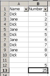
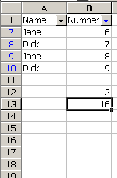
The range on the left is unfiltered. The range on the right is filtered on the Number column for Top 4.

The formulas are:

B12: =SUM((Rge1="Dick")*(SUBTOTAL(3,OFFSET(Rge2,ROW(Rge2)-MIN(ROW(Rge2)),,1))))

B13: =SUM((Rge1="Dick")*(SUBTOTAL(9,OFFSET(Rge2,ROW(Rge2)-MIN(ROW(Rge2)),,1))))

The OFFSET function used with SUBTOTAL returns an array which can be used as one element of an array formula. SUBTOTAL without OFFSET returns only a scalar value, not an array. These formulas not only limit based on “Dick” being in the name column, but also on the row being unfiltered.

In order to create a macro that modifies code, you need to set a reference to the Microsoft Visual Basic for Applications Extensibility Library. Chip Pearson has some great pages dealing with this library Programming to the Visual Basic Editor.

Jake asks:

I have a several ( 14 ) templates which contain an incorrect reference within the VBA, I would like to fix by sending out sheet which contains VBA to fix the incorrect reference.

Okay, that’s not really a question, but there was a question in the email. I swear.

I’m probably not the guy to be giving anyone advice on changing references programmatically. I don’t think I’ve ever had to do it. My workbooks are used in an environment that I pretty much control, so I don’t have a lot of problems with references. But I gave it a shot anyway. I’m sure if there are better approaches, someone will let me know in a comment.

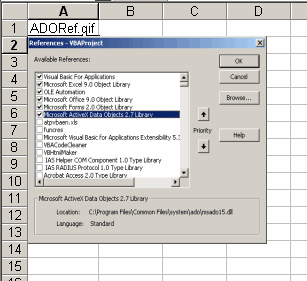
This assumes that you have a reference to a certain version of ADO and you want to change it to version 2.8. There’s probably no reason to actually do that, but that’s what I’m going with. I put the path to new library in a variable. I got this path by going to Tools > References, but it will no doubt be different on every machine. So what’s a good way to add that reference? AddFromGUID is probably better after you’ve scoured the registry with APIs, but if that’s so, I’ll let someone else figure that out.

I use a loop to remove the old reference, searching for a unique string in the Description. I could have also looked at the Name and deleted any with the name ADODB. As long as you’re scouring the registry for the new reference, I suppose you can get some info on the old reference and forget about the loop.

Other than telling you to set a reference and showing you the VBProject and Reference objects, this post sucks. Hopefully it will serve to provide better approaches via the comments.

Bill won the first anniversary contest and selected a copy of Professional Excel Development as his prize. He graciously agreed to send a picture, and here it is. Enjoy the book, Bill, and thanks for reading.

My wife and I split duties when it comes to teaching our kindergarten-age son. She teaches him reading and writing and I teach him math. To that end, I created a table to help him memorize adding and multiplying zero through nine. It’s nothing fancy, but you can have it if you like.

Download MathGames.zip

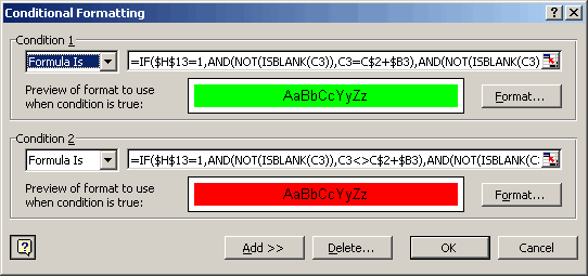
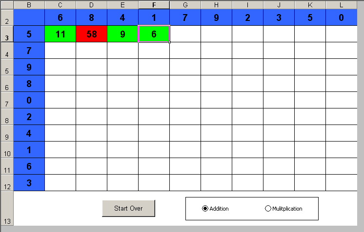
I started with a grid and some formatting. I use Row 1 and Column A to hold random numbers so I can sort Row 2 and Column B. The data entry grid is conditionally formatted to show green for correct answers and red for incorrect.

The formula for the first one is

The second formula is the same except for it’s ‘not equal’ instead of ‘equal’.

The Start Over button just resets everything with a simple macro:

I need to put some fancy animation in for when all the cells are green. So that there’s a prize for completing it.

A question from Chris:

[W]hat I would like to do is paste (link) a web image into a cell, the choice of web image dependent on another cell.

Eg. A1=îimage1î, paste http://web.com/image1.jpeg into A2

Here’s a macro that uses the AddPicture method of Shapes collection object.

The end result looks like this: