I bought a couple of books for my brother last week, but he’s misplaced his checkbook and couldn’t send the money. Sound like your brother? Maybe. J In this case, Doug decided to send the money using PayPal. He insisted that I receive the entire $85 he owed after PayPal took its cut, overestimated the fees, and sent me a couple of dollars more than the books cost. It’s no big deal, but I thought it would be interesting to put together a quick Excel worksheet that enables you to calculate how much you need to send so a recipient gets the proper payment after an intermediary deducts its fees.
The problem with this type of calculation is that it requires trial and error to find the proper value. As an example, consider the following worksheet:
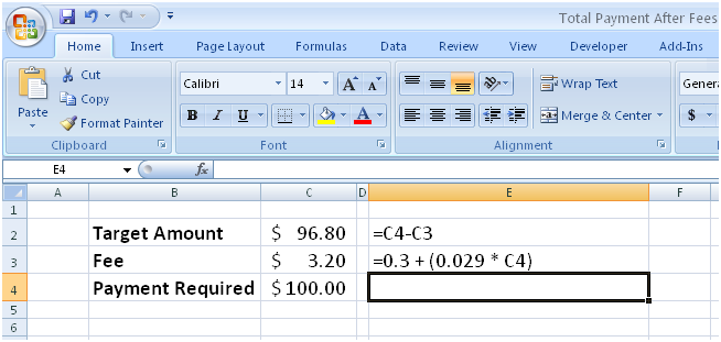
Cell C2 contains the amount the recipient gets after fees, cell C3 calculates the fee (in this case, $0.30 plus 2.9% of the payment), and cell C4 displays the amount you have to send to make cell C2 come out to the right amount. Sure, you could plug values into cell C4 until you get the desired result, but you can also use Goal Seek to have Excel do the work for you.
To start Goal Seek in Excel 2007, display the Data tab and then, in the Data Tools group, click What-If Analysis, and then click Goal Seek (in Excel 2003, open the Tools menu and click Goal Seek). The Goal Seek dialog box appears.
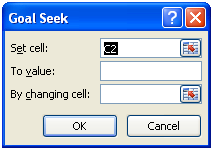
Type the address of the cell you want to set to a target value in the Set Cell field (C2), type the target value in the To Value field (in this case, 100), and then type the address of the cell Excel needs to vary to find the target value in the By Changing Cell field (C4). When you click OK, Goal Seek attempts to find an input value that produces the desired result. In this case, it was able to find a solution.
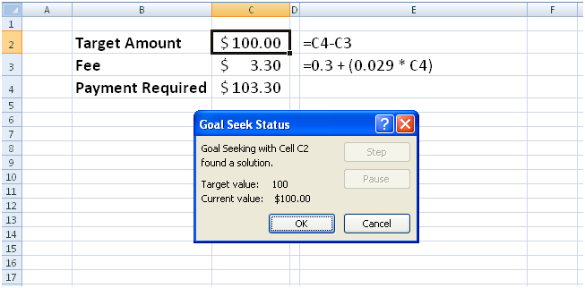
Click OK to retain the value in the worksheet, or click Cancel to return the worksheet’s previous values.

