Counting Unique Entries – Part 1

Editor’s Note:This is the last post created by Frank Kabel before his untimely death. I found it in the unpublished drafts bin and can’t think of any reason not to post it. So here it is:

One question which frequently appears in the Excel NGs is how to count unique entries. The following is an excerpt from a White Paper Bob Phillips and I created together.

As typical for Excel there’s not only one single formula to achieve this goal but several. Some of the most common ones are presented below:

  1. Formula: =SUM(IF(FREQUENCY(IF(LEN(A1:A10)>0,MATCH(A1:A10,A1:A10,0),””),IF(LEN(A1:A10)>0,MATCH(A1:A10,A1:A10,0),””))>0,1))
  2. Formula: =SUMPRODUCT((A1:A10<>””)/(COUNTIF(A1:A10,A1:A10&””)))
  3. Formula: =SUMPRODUCT((A1:A10<>””)/(COUNTIF(A1:A10,A1:A10)+(A1:A10=””)))

Notes:

  • Formula (1) is an array formulas entered with CTRL+SHIFT+ENTER.
  • All formulas ignore blank cells and zero length strings (=””)
  • All formulas can deal with mixed type of data (e.g. numbers, strings, etc.)
  • Formula (2) is only completely robust starting with Excel 2003. In previous versions you have to be sure what the data range (in our example A1:A10) is completely within the used range of your spreadsheet. Otherwise this formula returns #DIV/0. You can check this in a new/fresh workbook by simply entering this formula. To prevent this bug use formula (3) instead

Looking at the performance of these formulas formula (1) is much faster than the other two formulas (nearly 4-5 times faster). So my recommendation would be to use formula (1) if performance is an issue or formula (3) if performance is not that important for you and you don’t want to use an array formula.

If you want to learn more about these formulas (how they work, detailed benchmarks, etc.) you may have a look at the above mentioned White Paper.
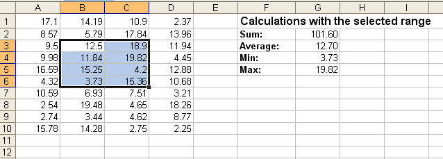
Calculating with the selected range

Jan Karel inspired me with his use of Excel4 Macros to Refer to the previous sheet and to determine page numbers to use this “old” Excel feature for something else: Automatic calculations with the current selected range.

To start first define the name Sel_Range with the formula:
=MID(CELL(“address”,($A$1,SELECTION())),6,255)&TEXT(NOW(),””)

Sel_Range returns a string representing the current selected range. Using INDIRECT this string can be converted to a range reference and used in the following type of formulas on your sheet:
=SUM(INDIRECT(Sel_Range))
=AVERAGE(INDIRECT(Sel_Range))
=MIN(INDIRECT(Sel_Range))
=MAX(INDIRECT(Sel_Range))

fk_selrange_1

Notes:

  • After entering this formula you first get a circular reference error. Just hit F9 after leaving the cell to refresh the formula result
  • To re-calculate the formula(s) simply press F9
  • And as always for using Excel4 macros: In versions prior to Excel 2003 DON’T copy formulas containing names using these macros as this will crash Excel

Happy new year
Frank Kabel

Replacing the Analysis Toolpak Addin – Part 4

This last part focusses on replacing some of the remaining functions of the Analysis Toolpak Addin (ATP). Reference to the other parts of this article series:

Other ATP functions
ATP Function Description ATP Syntax Replacement Formula Array formula
DELTA Test whether two values are equal =DELTA(number1,number2) =–(number1=number2) No
ISEVEN Returns TRUE if the number is even =ISEVEN(Number) =MOD(TRUNC(Number),2)=0 No
ISODD Returns TRUE if the number is odd =ISODD(Number) =MOD(TRUNC(Number),2)=1 No

So that is it. For the remaining ATP functions I currently have no replacement formula. If someone could provide corrections, additions I’m happy to amend the above tables accordingly.
Hope you find some of these formulas useful.

Frank

Replacing the Analysis Toolpak Addin – Part 3

This part focusses on replacing the numerical system conversion functions of the Analysis Toolpak Addin (ATP). Reference to the other parts of this article series:

Numeric System Conversion ATP functions
ATP Function Description ATP Syntax Replacement Formula Array formula
BIN2DEC Converts binary number to decimal =BIN2DEC(Number) =SUMPRODUCT(MID(“0″&Number,ROW(INDIRECT(“1:”&LEN(“0″&Number))),1)*2^(LEN(“0″&Number)-ROW(INDIRECT(“1:”&LEN(“0″&Number))))) No
BIN2OCT Converts binary number to octal =BIN2OCT(Number,Places) Combine solutions for BIN2DEC and DEC2OCT No
DEC2BIN Converts a decimal number to binary =DEC2BIN(Number) =SUMPRODUCT(INT(MOD(Number/2^(COLUMN(1:1)-1),2))*10^(COLUMN(1:1)-1)) No
DEC2OCT Converts a decimal number to octal =DEC2OCT(Number) =SUMPRODUCT(INT(MOD(Number/8^(COLUMN(1:1)-1),8))*10^(COLUMN(1:1)-1)) No
HEX2BIN Converts a hexadecimal to a binary =HEX2BIN(Number,Places) Combine solutions for HEX2DEC and DEC2BIN No
HEX2DEC Converts a hexadecimal to a decimal =HEX2DEC(Number) =SUMPRODUCT((MATCH(MID(“0″&Number,ROW(INDIRECT(“1:”&LEN(“0″&Number))),1),{“0″,”1″,”2″,”3″,”4″,”5″,”6″,”7″,”8″,”9″,”A”,”B”,”C”,”D”,”E”,”F”},0)-1)*16^(LEN(“0″&Number)-ROW(INDIRECT(“1:”&LEN(“0″&Number))))) No
HEX2OCT Converts a hexadecimal to an octal =HEX2OCT(Number,Places) Combine solutions for HEX2DEC and DEC2OCT No
OCT2BIN Converts an octal number to binary =OCT2BIN(number,places) Combine solutions for OCT2DEC and DEC2BIN No
OCT2DEC Converts an octal number to decimal =OCT2DEC(number) =SUMPRODUCT(MID(“0″&Number,ROW(INDIRECT(“1:”&LEN(“0″&Number))),1)*8^(LEN(“0″&Number)-ROW(INDIRECT(“1:”&LEN(“0″&Number))))) No

Missing functions: BIN2HEX, DEC2HEX and OCT2HEX as the creation of the characters A-F which are part of a hexadecimal number is not really feasible using worksheet functions.

Frank

Replacing the Analysis Toolpak Addin – Part 2

This part focusses on replacing the mathematical functions of the Analysis Toolpak Addin (ATP). Reference to the other parts of this article series:

Date ATP functions
ATP Function Description ATP Syntax Replacement Formula Array formula
EDATE Returns the Excel date / time serial number of the date that is the indicated number of months before or after the specified number of months from the start_date =EDATE(start_date,months) =DATE(YEAR(start_date),MONTH(start_date)+months,MIN(DAY(start_date),DAY(DATE(YEAR(start_date),MONTH(start_date)+months+1,0)))) No
EOMONTH Returns the Excel date / time serial number of the last day of the month before or after a specified number of months from start_date =EOMONTH(start_date,months) =DATE(YEAR(start_date),MONTH(start_date)+months+1,0) No
NETWORKDAYS Returns the number of whole working days between two dates excluding specified holidays =NETWORKDAYS(start_date,end_date,holidays) =SUMPRODUCT(–(WEEKDAY(ROW(INDIRECT(start_date&”:”&end_date)))<>1),(–(WEEKDAY(ROW(INDIRECT(start_date&”:”&end_date)))<>7)),–(COUNTIF(holidays,ROW(INDIRECT(start_date&”:”&end_date)))=0))*(1-2*(start_date>end_date)) No
WEEKNUM Returns the weeknumber in the year. The 1st week starts Jan-1; the 2nd week starts the following Sunday (return_type = 1) or Monday (return_type = 2).
Replacement formula returns the ISO weeknumber.
=WEEKNUM(serial_num,return_type) =1+INT((serial_num-DATE(YEAR(serial_num+4-WEEKDAY(serial_num+6)),1,5)+
WEEKDAY(DATE(YEAR(serial_num+4-WEEKDAY(serial_num+6)),1,3)))/7)
No
WORKDAY Returns the Excel date / time serial number of the date before or after a specified number of workdays excluding holidays =WORKDAY(start_date,days,holidays) =start_date+IF(days=0,0,SIGN(days)*SMALL(IF((WEEKDAY(start_date+SIGN(days)*(ROW(INDIRECT(“1:”&ABS(days)*10))),2)<6)*ISNA(MATCH(start_date+SIGN(days)*(ROW(INDIRECT(“1:”&ABS(days)*10))),holidays,0)),ROW(INDIRECT(“1:”&ABS(days)*10))),ABS(days))) Yes

Only missing function if this area is YEARFRAC as I consider this function ‘buggy’ anyway. For more about this read this newsgroup post of Norman Harker.

Frank

Replacing the Analysis Toolpak Addin – Part 1

The Analysis Toolpak Addin (ATP) is one of the most often used Excel Addins and provides several useful function. But the ATP has one major drawback: If internationalisation is an issue for you using the ATP will cause problems in your spreadsheets. Unfortunately Excel does not automatically translate the ATP functions to their local equivalents then opened in a different Excel language version but leaves the formulas unchanged. This will result in #NAME (or the local equivalent error message) errors in cells which make use of these functions.

Common recommendation is to not use ATP functions. But that is easier said then done. How to replace these useful functions if you don’t want to use VBA User Defined Functions instead? The following article therefore will provide alternative formulas for some of the ATP functions. As the ATP consists of 93 formulas (if I’ve counted them correctly) this article is divided in several ATP function areas:

I will not provide replacement formulas for all ATP functions (mostly due to lack of knowledge) but maybe someone else will step in and provide the remaining ones. Also I’m hoping for more efficient solutions for some of the replacement formulas I’ll present.

Mathematical ATP functions
ATP Function Description ATP Syntax Replacement Formula Array formula
BESSELJ Returns the Bessel function BESSEJ(x,n) =SUM(-1^(ROW(INDIRECT(“1:50”))-1)/(2^(2*(ROW(INDIRECT(“1:50”))-1)+ABS(INT(n)))*FACT(ROW(INDIRECT(“1:50”))-1)*FACT(ABS(INT(n))+(ROW(INDIRECT(“1:50”))-1)))*x^(2*(ROW(INDIRECT(“1:50”))-1)+ABS(INT(n)))) Yes
DOLLARDE Converts a dollar price (expressed as a fraction) into a dollar price expressed as a decimal number =DOLLARDE(fractional_dollar,fraction) =TRUNC(fractional_dollar)+((fractional_dollar-TRUNC(fractional_dollar))*10)/fraction No
DOLLARFR Converts a dollar price (expressed as a decimal number) into a dollar price expressed as a fraction =DOLLARFR(decimal_dollar,fraction) =TRUNC(decimal_dollar)+((decimal_dollar-TRUNC(decimal_dollar))/10)*fraction No
ERF Returns the error function integrated between lower_limit and upper_limit =ERF(lower_limit,upper_limit) =GAMMADIST(upper_limit^2,0.5,1,TRUE)-GAMMADIST(lower_limit^2,0.5,1,TRUE) No
ERFC Returns the complementary ERF function integrated between x and infinity =ERFC(x) =ChiDist(2*x^2,1) No
FACTDOUBLE Returns the double factorial of a number =FACTDOUBLE(number) =PRODUCT(IF(MOD(ROW(INDIRECT(“1:”&number)),2)=MOD(number,2),(ROW(INDIRECT(“1:”&number))))) Yes
GCD Returns the greatest common divisor of 2 – 29 integers =GCD(number1,number2,…) =MAX(IF((MOD(number2,ROW(INDIRECT(“1:”&number1)))&MOD(number1,ROW(INDIRECT(“1:”&Anumber1))))=”00?,ROW(INDIRECT(“1:”&number1)))) Yes
GESTEP Tests whether a number is greater than a threshold value =GESTEP(number,step) =–(number>=step) No
LCM Returns the least common multiple of 1 – 29 integers =LCM(number1,number2, …) =number2*MATCH(0,MOD(number2*ROW(INDIRECT(“1:”&number1)),number1),0) Yes
MROUND Returns a number rounded to the desired multiple. Midway points are rounded away from 0 =MROUND(number,multiple) =ROUND(number/multiple,0)*multiple No
MULTINOMIAL Returns the ratio of the factorial of a sum of values to the product of factorials =MULTINOMIAL(number1,number2, …) =FACT(SUM(number1,number2,…))/PRODUCT(FACT(number1,number2,…)) Yes
QUOTIENT Returns the integer portion of a division =QUOTIENT(numerator,denominator) =TRUNC(numerator/denominator) No
RANDBETWEEN Returns a random number between (and inclusive of) two specified numbers =RANDBETWEEN(bottom,top) =INT((top – bottom + 1) * RAND() + bottom) No
SERIESSUM Returns the sum of a power series expansion =SERIESSUM(x,n,m,coefficients) =SUMPRODUCT(coefficients,x^(n+m*(ROW(INDIRECT(“1:”&ROWS(coefficients)))-1))) No
SQRTPI Returns the square root of a number multiplied by pi =SQRTPI(number) SQRT(PI()*number) No

So this is the first part. ATP functions for which I don’t have a replacement formula in this area are: All BESSEL functions. So feel free to add them :-)

Update 21-Dec-2004:
Asser was helpful in providing a worksheet formula for the BESSEJ function. So only 3 of the 4 Bessel functions remain

Frank

Concatenating and splitting strings

As processing strings with formulas is kind of fun just to add some more formulas for this.
1. Concatenating strings
As you probably already know Excel’s worksheet functions do not support string concatenation for an array. e.g. the following:
=CONCATENATE(A1:A10)
does not work. Typical suggestion in these cases would be to use a UDF (or an add-in such as MOREFUNC.XLL with the function MCONCAT).
For only small ranges you could still do it with worksheet functions. The problem is how to deal with blank cells if you want to use a delimiter between each filled cell and without checking each single cell for blank.

So let’s have a look at the following example:
fk_string_1

Formula used (in cell F1): =SUBSTITUTE(TRIM(A1&” “&B1&” “&C1&” “&D1),” “,”-“)

As you can see this formula concatenates (using the hyphen as delimter) the strings in column A-E and skips blank cells. This formula has one restriction though: The concatenated cells are not allowed to contain spaces. So if you need a more complex solution best to use VBA for this.

2. Splitting strings in characters
The following is probably more a fun application but if you want to split a string value into its single characters you can achieve this with the following formula:
fk_string_2

Formula used (in C1): = MID($A1,COLUMN()-COLUMN($C1),1)
and copy this formula across.

Frank

String manipulation with worksheet formulas – Part 2

Deutsche Version / German version

Now continuing the first part of string manipulations with formulas the following will describe how to extract the nth element of a larger string. This technique is for example useful in the following cases:

  • Extract first, middle and last name
  • Get the last or first word of a sentence (words separated by spaces)

As an assumption for the following I’d assume that words in a larger string are separated by spaces. e.g. “This is a longer text of words separated by spaces”
So now let’s start extracting the individual elements of this string

1. Getting the first element
Getting the first word is rather simple. Just combine the functions LEFT and FIND (and add some error checking):

=IF(LEN(A1)=0,””,IF(ISNUMBER(FIND(” “,A1)),LEFT(A1,FIND(” “,A1)-1),A1))

This formula searches for the first occurence of a space character and returns all characters to the right of this space. If no space character is found the complete string is returned. For our example this formula would return “This”.

2. Getting the last element
Now it’s getting a little bit more complicated as we don’t know in advance how many elements our string contains and Excel does not provide a FIND function which searches from the right (as you have in VBA with the method InStrRev). But is is still possible to achieve with formulas alone. We start with getting the position of the last delimiter (the last space character):

  1. Using SUBSTITUTE and FIND:
    =FIND(“^^”,SUBSTITUTE(” “&A1,” “,”^^”,LEN(” “&A1)-LEN(SUBSTITUTE(” “&A1,” “,””))))-1
  2. Using LOOKUP:
    =LOOKUP(2,1/(MID(” “&A1,seq,1)=” “),seq)-1
    where seq is again a defined name with the formula: =ROW(INDIRECT(“1:1024”))

Personally I prefer the second alternative as it is shorter (and for me easier to remember). But both formulas should return the same result. For our example theywill both return: 44
Now the only thing you have to do use this formula part within a MID formula (and don’t forget to add 1 to the position to skip the space):

  1. Using SUBSTITUTE and FIND:
    =MID(A1,FIND(“^^”,SUBSTITUTE(” “&A1,” “,”^^”,LEN(” “&A1)-LEN(SUBSTITUTE(” “&A1,” “,””))))-1+1,1024)
  2. Using LOOKUP:
    =MID(A1,LOOKUP(2,1/(MID(” “&A1,seq,1)=” “),seq)-1+1,1024)

Both formulas would return the string: “spaces”

Getting the nth element
Adapting the approach of SUBSTITUTE and FIND for getting the last element you could also get the position for the nth and n+1 element within a string. Using this you get a kind of ‘monster’ formula:

=IF(OR(LEN(A1)=0,ISERROR(FIND(“^^”,SUBSTITUTE(” “&A1,” “,”^^”,$B$1)))),””, MID(A1,FIND(“^^”,SUBSTITUTE(” “&A1,” “,”^^”,$B$1)),IF(ISERROR(FIND(“^^”,SUBSTITUTE(
A1,” “,”^^”,$B$1))),1024,FIND(“^^”,SUBSTITUTE(A1,” “,”^^”,$B$1)))-FIND(“^^”,SUBSTITUTE(
” “&A1,” “,”^^”,$B$1))))

where B1 stores the desired element number n.

And as stated in the first part of this article this could of course be achieved much easier using VBA but maybe it wouldn’t be that much fun …

Frank

Pages: 1 2