This stack overflow question is intriguing. The way icon sets works is that you select a range and each cell within that range is evaluated against the other cells in that range (or a hardcoded number). The percent or value you set can be a cell reference, but not a relative cell reference. Let’s look at an example. Here are 24 numbers over two years. I want an icon in all the 2015 cells that shows how it compares to the prior year.
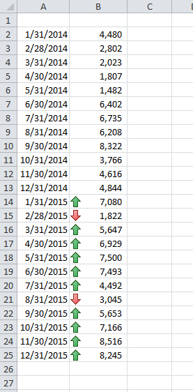
I set up a CF for B14 that looks at B2, but I can’t make B2 relative. It has to be absolute. Look at 7/31/2015. It’s less than 7/31/2014, but still shows an up arrow because it’s being compared to B2.
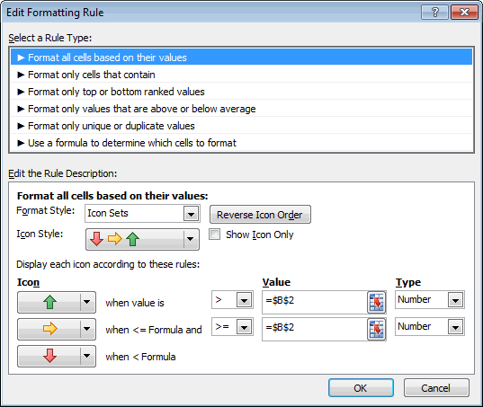
If I copy this down to the other months, the B2 remains – that’s how absolute works. If I copy B14’s formatting down to all the cells at once, I get two CF rules: one for B14 and one for B15:B25. If I copy the CF down one cell at a time, I get 12 CF rules, but they still all point to B2.
No problem. I’ll use a little
|
1 |
OFFSET |
trickery. I select B14:B25 and make a rule that says
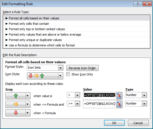
The relevant formula is
|
1 |
=OFFSET($B$2,ROW()-14,0,1,1) |
. You wants absolute references? I gots absolute references. No dice (I put some edge cases in there and copied the 2014 numbers down so I could see what was happening).
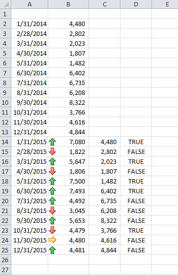
That should work, but it doesn’t. Instead of doing it to the whole range at once, I did that same CF to B14 only, then copied it down one cell at a time.
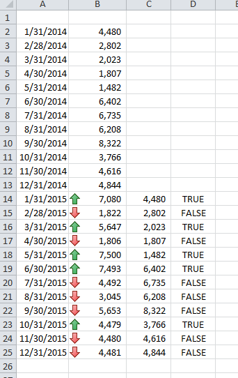
Et voilà! What a pain.
Thank you very much for this. I tried it in a regular worksheet and it works fine, however, when I try to do the same thing for the conditional formatting of a pivot table (comparing to the value of the previous month) it does not work. It shows arrows, but the direction/color does not correspond to the numbers at all. Do you have any idea why or even how to solve this?
Thanks, hadde
I’ve solved this in the past by avoiding Icon sets altogether and instead using custom number formats which contain arrows. So with my old friend character map find the arrows and set up three custom number formats something like:
↓* #,##0
→* #,##0
↑* #,##0
and associate with three appropriate formula based conditional formatting rules with relative referencing.
Late to the party — but I came across this post while working on a solution for an excel problem-solving forum.
I appreciate the suggestion. I wanted to add the observation that after using this technique to build a single column of cells with CF icons, I was able to apply the same CF rules to a second and third column as a batch, using Format Painter… So, I only had to do the cell-by-cell copying on a single column, not the whole spreadsheet.
Great. But If I need to refer not at the same cell.
Example, in your istruction you look at B2 value, but I need to look one cell up where I put the conditional formatting. Then when i put the conditional formatting in the next cel (1 row down) I need to look the cell up (1 row up). This for all the column.
CAn i do this ?
Thanks
Germano: If you have data in A4:A25, for example, then you would use
In A5 and copy that down cell-by-cell. If your data starts in a different cell, the 5 would have to change. I guess you could use
so that it would change automatically as you insert rows.
Thank you very much that is awesome
I went across the lack of ability to use relative reference differently. In my case, the data was aligned in pairs of cells scattered across a sheet (i.e. C2 & D2). First cell was Forecast and second cell was Actual. And the requirement was to show one of the 3 colored icons if Actual was above forecast, if it was equal to Forecast or up to 90% of it, or if it was below 90% of the forecast. I used ADDRESS nested within INDIRECT and applied the formulas as follows:
(a) =INDIRECT(ADDRESS(ROW(),COLUMN()-1))
(b) =0.9*INDIRECT(ADDRESS(ROW(),COLUMN()-1))
These formulas always refer to the adjacent cell to the left. After I copy-pasted the initial conditional formatting rule configured, I pasted it over all the Actual cells. The only caveat of this method, is that when you copy and paste-special the formatting, you end up with individual conditional formatting rules as the number of pastes that you do. Unfortunately this solution of dynamic reference can only be used on one cell at a time (per conditional formatting rule).
How do I adjust this to my table if I completely fail to understand said OFFSET trickery?