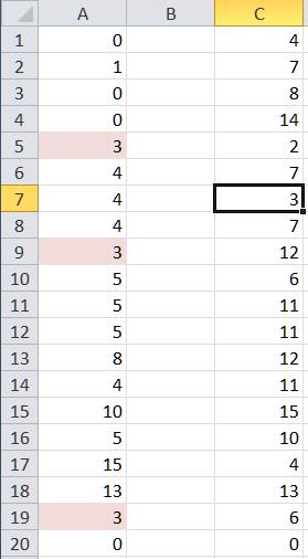
I came across a very reasonable request from someone who wanted to see which entries in a list matched those in the current cell (http://answers.microsoft.com/en-us/office/forum/office_2010-excel/event/49aa9987-3cf5-4007-9f08-df076ff0beba). While the original request dealt with names, I abstracted the problem into a set of numbers. Column A in Figure 1 is one list of numbers. Column C represents a list that we want to check against column A. Selecting a cell in column C should highlight all the matches in column A.

Figure 1
For a version in a page by itself (i.e., not in a scrollable iframe as below) visit http://www.tushar-mehta.com/publish_train/xl_vba_cases/0702 Highlight matches to current cell.shtml
Being lazy here, but how might one modify the code to only recalculate on selection change for a specific range? For example, in your sample worksheet, limit the “monitored” cells to the range A1:A20. That way, unnecessary recalculations aren’t being initiated…
Not too complicated I suppose:
Target.Name = “tst”
If Target.Column = 3 And Target <> “” Then Range(Join(Filter([transpose(if(A1:A100=tst,address(row(A1:A100),1),“”))], “$”), “,”)).Select
End Sub
That is actually very cool and can be a great tool in meetings that involve Excel. Gret for presentations, but also great for analysis. It really saves the brain and the eyes.
Christopher
I like the conditional formatting formula. I modified it to highlight a specific cell in the same row. However it did not automatically highlight the cell because my calculation is set to manual. I had to add the “Calculate” command right after the “Target.Calculate” in the code module. Then it worked for me.
Hi Tushar
That’s a cool trick.
Just nit-picking but I just use the TRUE condition for Conditional Formatting.
So
should work.
To my eyes, I’d like to see cells in Column A with matching values highlighted only when cells in Column C are selected, otherwise show without formatting.
So I would use 2 conditonal formats.
The “shady” one would be
And the “clear” one with no formatting would be
.
The Worksheet_SelectionChange code would calculate the entire sheet but to make it range specific, I could use something like
If Not Intersect(Target, Range(“A1:F20”)) Is Nothing Then Range(“A1:F20”).Calculate
End Sub
Hope I got the vb tags right :-)
Hi Tushar,
we can add *Now() to calculate instade of Worksheet_SelectionChange
=IF(CELL(“col”)=COLUMN(C:C),A1=CELL(“contents”),FALSE)*NOW()
Tushar
Please ignore my previous comment.its my mistake.
Sudhir.