Did you ever need a worksheet function to determine if a range is sorted? Neither have I. But I’m all about answering questions that haven’t been asked.
=SUMPRODUCT(--(A1:A10>=A2:A11))=--(A11<A10)
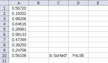

The SUMPRODUCT part compares every cell in the range to the one below it. If any cell is greater than the one below it, it returns TRUE and the double unary converts that to a 1. In this example, the SUMPRODUCT will return 1 – all cells are less than the one above it except A10 which is greater than A11 (blank).
That brings us to the right side of the equation. If A11 is less than A10 (as it is in this example), the expression will evaluation to TRUE. Again the double unary coerces the Boolean into a 1. If A11 happened to be greater, it would return FALSE, or zero. We don’t really care if A11 is sorted, but we use the fact of whether it is to compare to the SUMPRODUCT result. If A11 is sorted, SUMPRODUCT will return zero for an otherwise sorted list. If not, SUMPRODUCT will return 1. If anything else if not sorted, SUMPRODUCT will return a larger number and the whole expression will be false.
Up in the formula bar, I use Control+= (or F9) to evaluate portions of the formula
=SUMPRODUCT(--({FALSE;FALSE;FALSE;FALSE;FALSE;FALSE;FALSE;FALSE;FALSE;TRUE}))=--(A11<a10 )

=SUMPRODUCT({0;0;0;0;0;0;0;0;0;1})=--(A11<A10)

=1=--(A11<A10)

=1=--(TRUE)

=1=1

TRUE
Any reason not to use the more obvious AND solution? Yeah, it’s an array formula but it’s soooo much more obvious. {grin}
Not to mention that it will work even with data on the last row of the worksheet (yeah, like that’s ever happened to me).
Suppose the data are in B2:B6. Then the *array*(1) formulas
=AND(B2:B5< =B3:B6) indicates an ascending order.
=AND(B2:B5>=B3:B6) indicates a descending order.
=OR(AND(B2:B5< =B3:B6),AND(B2:B5>=B3:B6)) indicates either an ascending or a descending order.
Remove the = to get strict order.
And with the named formulas below, the result adjusts to a changing data range.
aRng=OFFSET(Sheet1!$B$2,0,0,COUNTA(Sheet1!$B:$B),1)
aRng1=OFFSET(aRng,0,0,ROWS(aRng)-1,1)
aRng2=OFFSET(aRng,1,0,ROWS(aRng)-1,1)
=OR(AND(aRng1>=aRng2),AND(aRng1<=aRng2))
(1) For those who might be new to array formulas, to complete an array formula use the CTRL+SHIFT+ENTER key combination and not just the ENTER or TAB key. If done correctly, Excel will show the formula enclosed in curly brackets { and }
Handy!
Define
Lst = =’1′!$A$1:INDEX(‘1’!$A:$A,COUNTA(‘1’!$A:$A)-1)
LstOff =’1′!$A$2:INDEX(‘1’!$A:$A,COUNTA(‘1’!$A:$A))
Sort =AND(AND(Lst<=LstOff)AND(Lst>=LstOff))
Works for both Asc and Desc
Thanks for this! We were working with a large spreadsheet and wanted an easy way to conditionally format the column that was being sorted – and we had to do it without VBA or macros due to security settings. This was exactly what we needed.
This is an awesome formula (and also works for text!). However, it doesn’t work when there is a duplicate number (or text) in the data. Is there a modification that might solve that? Thanks!
This seems to work if there are duplicates.
=SUMPRODUCT(--(A1:A10>A2:A11))=--(A11<A10)That does it, thanks!!
Although now I’m seeing that it won’t work if there are blanks? Any ideas on that?
This will work with blanks I think.
=SUMPRODUCT(--(A1:A10<=A2:A11))=COUNT(A1:A10)-1That latest one doesn’t seem to be working for blanks. I’m thinking this would require creating a temporary list in the array function that excludes blanks, no matter how many (for, say rows 1:10), and then compare that to the same logic applied to say, rows 2:11?
When I say a temporary list, I mean creating those two lists “in the formula” without having to use a helper column, if that’s possible. Thanks again!
It works for blanks unless the blank is the first or the last cell. I didn’t test the extremes, I guess. This seems to work for any blanks
=SUMPRODUCT(--(A1:A10<=A2:A11))=COUNT(A1:A10)-1+ISBLANK(A10)+ISBLANK(A1)Nope. That won’t work if the first two are blank.
This might work for numbers, but not text
{=INDEX(RANK.EQ(A1:A10,A1:A10,1),MAX((NOT(ISBLANK(A1:A10))*ROW(A1:A10))))=SUM((A1:A10<>"")/COUNTIF(A1:A10,A1:A10&""))}