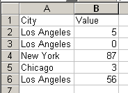
I’ve discussed MAXIF and MINIF previously, but using MIN in an array formula can be tricky. Mike provided another example that I thought was worth sharing.

To find the MAX value for Los Angeles is pretty straight forward.
=MAX((A2:A6=”Los Angeles”)*(B2:B6))
For any entry in A2:A6 that is not Los Angeles, the array will contain zero so the MAX function automatically takes care of it.
The next part was the tricky part, or so it seemed. Find the MIN value for Los Angeles but only for non-zero values. For that, you need to wrap the whole array in an IF statement and convert any zeros into strings so they are ignored by the MIN function. What makes this less tricky is the fact that non-Los Angeles entries will be zero (and we want to ignore those) and zero entries will be zero (and we want to ignore those). So all the rows that we want to ignore are zero. Here’s the formula
=MIN(IF((A2:A6=”Los Angeles”)*(B2:B6)=0,””,B2:B6))
I really got twisted around on that one, but I suppose even the failures are useful. To use my failing effort, suppose that you want to find the MIN for Los Angeles but only for values that are greater than 5. Now it’s not true that all of the rows I want to ignore will be zero, so there’s one extra step involved.
=MIN(IF((A2:A6=”Los Angeles”)*(B2:B6>5)*(B2:B6)=0,””,B2:B6))
You can probably guess how I over-complicated the first MIN. Oh well, live and learn.
Hi Ken
why not use for
=MIN(IF((A2:A6=”Los Angeles”)*(B2:B6>5)*(B2:B6)=0,””,B2:B6))
instead the following formula :-)
=MIN(IF((A2:A6=”Los Angeles”)*(B2:B6>5),B2:B6))
FALSE boolean values are also ignored by MIN/MAX. Same applies for the second formula:
=MIN(IF((A2:A6=”Los Angeles”)*(B2:B6<>0),B2:B6))
Equivalent to
=MIN(IF((A2:A6=”Los Angeles”)*(B2:B6>5),B2:B6))
but simpler:
=SUM((a2:a6=”Los Angeles”)*(b2:b6>5)*(b2:b6)).
=MIN((a2:a6=”Los Angeles”)*(b2:b6>5)*(b2:b6))
would be even better
(formula result in previous comment turned out to be correct because of small # of LA-values)
The point is that in order to obtain a conditional result from a table, there is no need to use the IF-function, only multiplication of the conditions with each other.
Frank K: I don’t know who Ken is, but I love that MIN ignores FALSE. Very cool.
frank (not Kabel): I don’t think that second MIN function works. If any entries are not Los Angeles, they will return zero and that will be the MIN. Am I missing something?
I put my hand over my mouth. Though I have spoken once, I will not do so again; though twice, I will do so no more.
(Book of Job 38,1.12-21.40,3-5.)
Who can beat Ken Wright and Frank Kabel on conditional array formulas? I still think their approach is too little understood. See also
http://www.xldynamic.com/source/xld.SUMPRODUCT.html#top
Excel isn’t letting me do this. It keeps pointing to the text value criteria (e.g. =”Los Angeles”) as the problem. I tried adding a column and assigning a numeric value to each text string, and making the if statement if(range=3)*(2nd range), but I get the same error. I’m going to look for your other articles of minif and maxif and see if I get any help. I find it odd that you would publish something that doesn’t work.
Nancy,
These are all examples of array formulas. You must enter them with Ctrl+Shift+Enter instead of just hitting Enter. They should work when you do that.
Excel 2007 doesn’t seem to support the CSE function (hitting Ctrl+Shift+Enter). It has SUMIF, but I haven’t found anything to make MINIF/MAXIF work.
Thijs – Array formulas do work in Excel 2007, including the ones given here.
I have multiple employee ID numbers along with what week they had their first sale. Is there a formula that I could enter in a column that would say for each employee ID what week they made their first sale? For example, employee ID 7050 had their first sale in week 3, employee 6321 made their first sale in week 4?
I’m just looking for a formula, I did not want to have to sort, filter or create a pivot table.
ID – WK
7050 – 6
7050 – 3
7050 – 4
6321 – 6
6321 – 4
6321 – 7
tom c: =MIN(IF((A2:A7=7050),(B2:B7)))
Is it possible to use the MIN(IF… functihon in Conditional Formatting? I can’t figure it out. Say, in your example above, I want to hilight the Minimum value in column B that has Los Angeles in Column A. (e.g. row 2 or 3 depending on if you want to exclude 0’s or not)
Thoughts?
Array formula worked perfectly for me in Excel 2007.