You can nest functions inside Excel formulas, but it’s limited to 7 levels of nesting. Nested formulas look something like this
=IF(A1=”One”,1,IF(A1=”Two”,2,IF(A1=”Three”,3,IF(A1=”Four”,4,IF(A1=”Five”,5,IF(A1=”Six”, 6,IF(A1=”Seven”,7,IF(A1=”Eight”,8,”N A”))))))))
If you wanted to test for Nine, you’d be out of luck. There are a few techniques for getting around that limt. Matthew sent me a couple that are worth sharing.
- Don’t use CONCATENATE – The ampersand (&) works the same as the function and doesn’t count against you.
- Put repeated part of your formulas in a Name
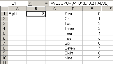
- Use VLOOKUP and put some data in a separate table
The above formula could be reduced with a table like this

For another example, take this formula
=INDIRECT(CONCATENATE(“Sheet1!B”,ROW()-1))
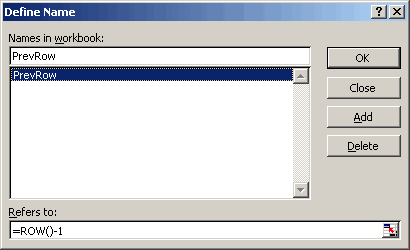
While not at the limit, it has two levels of nesting. If it was part of a larger formula, it could put the formula over. You can reduce the nested levels of this formula to zero by eliminating CONCATENATE and defining a name for the ROW()-1 part.

=INDIRECT(“Sheet1!B” & PrevRow)
Thanks for the tip and the great examples, Matthew.
Your example of nested IF() statements can be stated in an alternate way which then can be extended past the 7 nest limit.
=IF(A1=”One”,1,0)+IF(A1=”Two”,2,0)+IF(A1=”Three”,3,0)+IF(A1=”Four”,4,0)+IF(A1=”Five”,5,0)+IF(A1=”Six”,6,0)+IF(A1=”Seven”,7,0)+IF(A1=”Eight”,8,0)+IF(A1=”Nine”,9,0)+IF(A1=”Ten”,10,0)+IF(A1=”Eleven”,11,0)+IF(A1=”Twelve”,12,0)+IF(A1=”Thirteen”,13,0)+IF(A1=”Fourteen”,14,0)+IF(A1=”Fifteen”,15,0)+IF(A1=”Sixteen”,16,0)+IF(A1=”Seventeen”,17,0)+IF(A1=”Eightteen”,18,0)+IF(A1=”Nineteen”,19,0)+IF(A1=”Twenty”,20,0)….
This works best when using these types of comparisons.
Granted setting up a VLOOKUP table is better, but you either need to set the table up in another worksheet or some obscure part of the current worksheet so that it doesn’t get edited/deleted accidently.
Just my $.02 worth. :-)
Darn. I came up with something almost identical to Nick, but it posted to the wrong blog entry. Although mine differs from Nick’s as it eliminates the IF statement altogether. My original comment:
What about boolean gates? I was somewhat surprised they didn’t get a mention. A formula along the lines of:
=(A1=”One”)*1+(A1=”Two”)*2+(A1=”Three”)*3+(A1=”Four”)*4+(A1=”Five”)*5+(A1=”Six”)*6+(A1=”Seven”)*7+(A1=”Eight”)*8+(A1=”Nine”)*9+(A1=”Ten”)*10
…provides the ability to test beyond the nesting limit. I’m not suggesting for a moment that it’s pretty (I would normally use the method you suggested of a VLOOKUP table), but it works. And (IMHO) it’s a lot easier to follow than nested IFs as the logic is sequential instead of jumping all over the place, spaghetti code style.
I’ve also found in my travels that OR can help you get around using IFs to their limit, such as:
IF(OR(A1=”One’,A1=”Two”,A1=”Three”,A1=”Four”,etc),””,A1)
Here’s a way I thought up (seems to work, fingers crossed)
=IF(OR(A1={“Eight”;”Five”;”Four”;”Nine”;”One”;”Seven”;”Six”;”Ten”;”Three”;”Two”}),LOOKUP(A1,{“Eight”;”Five”;”Four”;”Nine”;”One”;”Seven”;”Six”;”Ten”;”Three”;”Two”},{8;5;4;9;1;7;6;10;3;2}),”No Criteria Found”)
The criteria to be matched are in alphabetical order so the LOOKUP function works properly.
Working off the cross-reference table, you could also use the following (entered as an array formula):
{=SUMPRODUCT(IF(A1=D1:D10,1,0),E1:E10)}
or as a standalone function (also an array formula):
{=SUMPRODUCT(IF(A1={“Zero”;”One”;”Two”;”Three”;”Four”;”Five”;”Six”;”Seven”;”Eight”;”Nine”},1,0),{0;1;2;3;4;5;6;7;8;9})}
Nesting IF’s is ugly. If you nest to 7 levels deep, by the time you come to placing the last few sets of brackets, my mind is spinning. Also, and more important, it is very difficult to edit later.
Along the lines already mentioned … I use both AND and OR. Eg If(AND(A2>77, A2<101, B2<>”Blue”)=true,[whatever],[whatever else] ). Here, we test for 3 conditions, but you can have 30ish. Furthermore, the syntax is so much easier, you can troubleshoot or edit months later.
Please mail me complex problems & their solutions for multiple nesting functions ( combination of if, or, and functions.
thanks
Aloha: I’m trying to set up a nested formula with 13 levels (for grading with “+” and “-“). I’ve tried a couple of your suggestions here as well as some of my own concoctions. I still can not get it to produce what I need. Basically, I want to be able to change a student’s numerical grade (e.g., 88.5) to a letter grade (e.g.,”B+”). Any suggestions? Mahalo. Bill
=IF(F5>96.4,”A+”)+IF(F5>92.4,”A”)+IF(F5>89.4,”A-“)+IF(F5>86.4,”B+”)+IF(F5>82.4,”B”)+IF(F5>79.4,”B-“)+IF(F5>76.4,”C+”)+IF(F5>72.4,”C”)+IF(F5>69.4,”C-“)+IF(F5>66.4,”D+”)+IF(F5>62.4,”D”)+IF(F5>59.4,”D-“)+IF(F5<59.5,”F”)
Hi
for this kind of application use VLOOKUP and a lookup table. e.g. in column A and B enter:
A B
1 0 F
2 59.5 D-
3 62.5 D
4 66.5 D+
….
Now use a formula such as
=VLOOKUP(F5,$A$1:$B$20,2,TRUE)
Frank
Thanks Frank. While I was waiting, I found another website at Ball State Univ. Tung Liu provided this solution. Rather cumbersome but it worked. I’ll have to try your suggestion as well.
http://web.bsu.edu/tliu/faq/
=IF(E5>=72.5,
IF(E5<76.5,” C”,IF(E5<79.5,” C+”,
IF(E5<82.5,” B -“,IF(E5<86.5,” B”,IF(E5<89.5,” B+”,
IF(E5<92.5,” A -“,IF(E5<96.5,”A”,”A+”))))))),
IF(E5>=69.5,” C -“,IF(E5>=66.5,” D+”,
IF(E5>=62.5,” D”,IF(E5>=59.5,” D -“,” F”)))))
Bill
I forgot to mention that I had to modify Tung Liu’s formula a bit for my grading system.
Bill
Bill –
What happens if you change the cutoff values for the grades? Dozens of formulas will have to be changed. Sure, you can just copy-paste, but you may miss one, and someone misses an A because of a clerical error.
The nice thing about a lookup table like Frank’s is that you can see at a glance what the cutoffs are, and you only have to make a change in one place instead of everywhere the logic is invoked.
– Jon
The way to nest Dick’s first formula more efficiently is to break each if into roughly equal pieces. His first IF,
IF(A1=”One”
breaks the problem into “One” and {Everything Else}. In the complex formula below, I’ve broken the problem into {“Zero”,”One”,”Two”,”Three”,”Four”} and everything else. Then I break this into {“Zero”,”One”} and the rest of {“Zero”,”One”,”Two”,”Three”,”Four”}, which is {“Two”,”Three”,”Four”}. And so on. Here’s the formula:
=IF(OR(A1={“Zero”,”One”,”Two”,”Three”,”Four”}),IF(OR(A1={“Zero”,”One”}),IF(A1=”Zero”,0,1),IF(OR(A1={“Two”,”Three”}),IF(A1=”Two”,2,3),4)),IF(OR(A1={“Five”,”Six”,”Seven”,”Eight”,”Nine”}),IF(OR(A1={“Five”,”Six”}),IF(A1=”Five”,5,6),IF(OR(A1={“Seven”,”Eight”}),IF(A1=”Seven”,7,8),9)),”No Match”))
I don’t know how many levels I’ve nested, but I think I could go further without too much trouble. It’s still not as quick or easy as building a lookup table, but it shows a way to nest the formula more efficiently.
Here’s what I get in the worksheet:
Zero0
One1
Two2
Three3
Four4
Five5
Six6
Seven7
Eight8
Nine9
ElseNo Match
– Jon
Jon, thanks for the comment. I’ve elected to go with Frank’s suggestion of using the VLOOKUP command. I had to tweak it slighty from .5s to .4s But it’s working just fine.
Bill
Get Past the 7 Nested IF limit
I need to implement a more than 7 IF nested Statements in a Master Excel sheet I am creating. It is a Tolerance Table that I need to put several times across the sheet and across the book. I know it can be done in VBA but I am not an expert in VBA.
Of course I tried to write the whole formula in EXCEL although I know it was not going to be accepted.
Average % intervalsTolerance
99and22
97-98and4-Mar3
94-96and7-May4
91-93and10-Aug5
87-90and14-Nov6
82-86and15-197
76-81and20-258
70-75and26-319
60-69and32-4110
51-59and42-5011
=IF(CELL=2,”2?,IF(CELL
I was wondering if there is any way to increase the amount of conditional formats in a worksheet beyond 3? Thanks
I’m working around this formula (it’s in Portuguese: SE=IF;E=AND; PROC=FIND):
=SE(É.ERRO(SE(E(G108=”INF A”;B108=”M”);PROC(F108;{0;1954;2100;2395;2544;4000};{1;2;3;4;5});SE(E(G108=”INF A”;B108=”F”);PROC(F108;{0;1954;2100;2395;2544;4000};{1;2;3;4;5});SE(E(G108=”INF B”;B108=”M”);PROC(F108;{0;1954;2100;2395;2544;4000};{1;2;3;4;5});SE(E(G108=”INF B”;B108=”F”);PROC(F108;{0;1728;1844;2075;2191;4000};{1;2;3;4;5});SE(E(G108=”INIC”;B108=”M”);PROC(F108;{0;2016;2207;2589;2780;4000};{1;2;3;4;5});SE(E(G108=”INIC”;B108=”F”);PROC(F108;{0;1759;1874;2102;2217;4000};{0;1;2;3;4;5});SE(E(G108=”JUV”;B108=”M”);PROC(F108;{0;2271;2416;2706;2851;4000};{1;2;3;4;5});SE(E(G108=”JUV”;B108=”F”);PROC(F108;{0;1743;1854;2078;2189;4000};{1;2;3;4;5});SE(E(G108=”JUN”;B108=”M”);PROC(F108;{0;2084;2320;2795;3034;4000};{1;2;3;4;5});SE(E(G108=”JUN”;B108=”F”);PROC(F108;{0;1593;1689;1881;1977;4000};{1;2;3;4;5}))))))))))));”-“;SE(E(G108=”INF A”;B108=”M”);PROC(F108;{0;1954;2100;2395;2544;4000};{1;2;3;4;5});SE(E(G108=”INF A”;B108=”F”);PROC(F108;{0;1954;2100;2395;2544;4000};{1;2;3;4;5});SE(E(G108=”INF B”;B108=”M”);PROC(F108;{0;1954;2100;2395;2544;4000};{1;2;3;4;5});SE(E(G108=”INF B”;B108=”F”);PROC(F108;{0;1728;1844;2075;2191;4000};{1;2;3;4;5});SE(E(G108=”INIC”;B108=”M”);PROC(F108;{0;2016;2207;2589;2780;4000};{1;2;3;4;5});SE(E(G108=”INIC”;B108=”F”);PROC(F108;{0;1759;1874;2102;2217;4000};{0;1;2;3;4;5});SE(E(G108=”JUV”;B108=”M”);PROC(F108;{0;2271;2416;2706;2851;4000};{1;2;3;4;5});SE(E(G108=”JUV”;B108=”F”);PROC(F108;{0;1743;1854;2078;2189;4000};{1;2;3;4;5});SE(E(G108=”JUN”;B108=”M”);PROC(F108;{0;2084;2320;2795;3034;4000};{1;2;3;4;5});SE(E(G108=”JUN”;B108=”F”);PROC(F108;{0;1593;1689;1881;1977;4000};{1;2;3;4;5}))))))))))))
It works fine on excel2007 but i can’t use in excel2003. Can someone help!? Thanks
Sorry, “PROC” function is “Lookup”!… Anyone?!
Thanks anyway, problem is solved!