Data Validation is great when you want to limit possible entries to a predefined list. Sometimes, however, you want that list to be different based on another cell. This posts shows you how to use Data Validation to condition one list based on the selection in another.
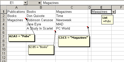
To do this, we need to set up some lists and name then using Insert>Name>Define. Here are some lists that I set up to illustrate.

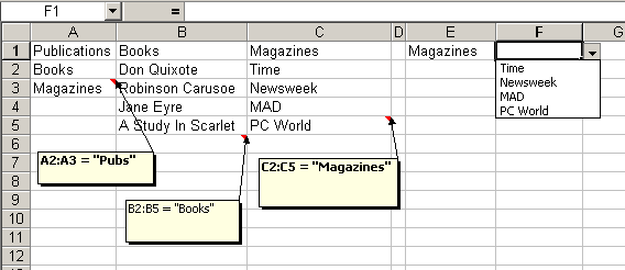
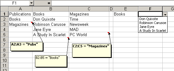
The comments at the bottom of the lists show what I’ve named them. The first name “Pubs” is unimportant. But the other two names match the entries in Pubs exactly. This is important as we’ll soon see. I’ve set up DV in cell E1 as shown in the comment to that cell. In E1, the user has the choice of Books or Magazines. Cell F1 also contains DV, but the choices in that list will depend on what is in E1. Here’s what the F1 lists look like for different E1 values.


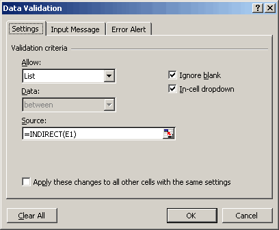
The DV in F1 is setup like this:

By naming the dependent ranges the same as the cells in Pubs, the INDIRECT function can be used to refer to them.
One cautionary note: If you change E1 after F1 has been selected, you’ll end up with a value in F1 that’s not in the appropriate list. No warning, no error, nothing. To alert users of this potential problem, consider adding conditional formatting to F1 to make it standout if the entry is not proper. Here’s one way you can do it.

NOTE: Make sure a value is selected in the INDIRECT reference cell before creating your INDIRECT list. If you don’t do this Excel will display an error.
Hi,
this solution for conditional formatting does not seem to work in Excel 2003.
Could you advise please?
Thanks,
Sarah
hi there,
is it possible to create a third level of contingent lists?
ie index of Time magazine?
regards
S Brijnath
Hi,
I can’t express my feelings. however i am very gald to get the right thing what i was looking for, from one week. best wishes for you and good luck.
Thanks & regards,
Atul sharma
Hello,
What was the answer to the question: Is it possible to create a third level of contingent lists?
Or is it possible?
This question was posted on July 29th, 2005 by S Brijnath.
Thank you,
Marty
Thank you very much! I was afraid that I was going to have to purchase a book that I kept getting referred to. :) This is a very clever fix to what appears to be a common need.
I, too, am very interested in a third level of a data validation dependent list. Does anyone know the answer? I have not seen it addressed positively or negatively on any of my usual sites…
Thanks and good day, G
Hi,
I was really really impressed. I have been looking for something like this for a couple of days and this one is really amazing.
Keep up the good work
Many Thanks
Sanjib
For those who are interested in seeing how to implement this kind of scheme using a relational database structure (and supporting multiple levels) see
Cascading queries
http://www.tushar-mehta.com/excel/newsgroups/cascading_dropdowns/index.html
For a Inter/Intra-net based solution, see
Building cascading queries
http://www.tmehta.com/krtest/index.asp
though this (the last) URL is almost certain to change at some point in the future.
Loved it.
Thanks
Is it possible to use conditional validation on a userform?
I had been using the following to achieve similar results:
=IF(COUNTIF(INDIRECT(G30),H30)=0,TRUE,FALSE)
Which works fine when testing in a sheet where two conditionals are entered (i.e. the third selection is dependant on the second, which in turn is dependant on the first). But when I enter this formatting in my ‘live’ sheet which was the trigger for me trying to find something to flag errors in validation, it always throws up an error.
I was interested to try this ISERROR solution aswell but it does exactly the same; the formatting works fine (even when used in 1000 rows across two columns) and saves fine, but on reopening Excel (2003 here) crashes and I lose everything.
I’m resigned to the fact there might be something else in the sheet that is causing it, but whatever it might be is beyond my ken.
Anyone have similar problems using this conditional formula formatting?
Also, in theory, is either method preferable in terms of speed/complication?
First, let me say “WOW”!! Awesome website. I start checking out other categories and almost forgot why I got here in the first place.
I am working with Excel 2003 (just recently upgraded from 97)
I am creating an excel workbook that will contain 8-10 User worksheets each the same except for different depts. There will be multiple uses of each of these worksheets. I have tried to keep the worksheet simiple for the user by have most of the entries come from drop-down lists. I designed a separate worksheet (within this workbook) which holds all the lists being referenced in the drop-downs. What I would like to do is, is on the List Worksheet, link certain cells within a list to another worksheet (still in the same workbook) to display a series of 6 to 8 cells of Detailed Information. I am able to create this link between the cell within the List worksheet and the Detail Info worksheet, however on the Users worksheet, when I test the cell which holds the drop-down list with the values link on the List worksheet, I only have plain text – no link?? Am I going about this the wrong way? Any Suggestions would be greatly appreciated. Please note when the workbook is complete, the List and Detailed Info worksheets will be locked and “well hidden”.
Thank you
Very nice tutorial. I was getting very frustrated trying to do this. Thanks for the help!
BEWARE!!
I get the same problem as Gordon (12) in Excel 2002; after putting the ISERROR in, saving, exitting and reopening, excel crashes.
Note: I just tried it on a simpler spreadsheet – no problem. hmm.
His workaround has an issue: it only applies formatting if F1’s value is a defined name.
Anyone know how to do this?
Does anyone have an answer to Margaret’s comment/question? I’ve had similar questions about displaying detailed information for single list entries and have begun to consider a few possible solutions; such as:
Using a Concatenate function that takes on an array to display at least some of the text.
Having a paste picture link situation in an Shape layer or in the comment.
Having the data from the two worksheets in separate external database files for filtered reference.
But none of these are simple or particularly more efficient than going to something like Access for a relational database.
Am I on the right track here?
Hi,
I have a similar problem. I need to get data from two lists, one dependent on the other. I have followed the above procedure, it works, but the problem is regarding addition of new items in the first list(the independent one). Is there a way that when a new item is added a similar named range is also added to the worksheet, so that, the new added item also appears in the independent list.
Will appreciate any and all help in this regard
Hi,
I’m trying the same in excel 2003, I always get an error “the source currently evaluates to an error.do you wish to continue?” I’m following the same steps as mentioned above…
Please help.
I tried this in XP as told here. It is not working. Kindly please help.
For those who are interested, the third level works exactly the same as the second. Setup the validations lists for each of the values on the second level and remember to name the lists properly (i.e. the name of the choice from the second level).
Good luck.
Hi,
I am trying to have third list but which is based on first list. That is i want two lists depend on the first item.
let’s say i have list of failure components in the first list, depends on that failure component i want its loaction(like which part of the component) and observation(Reason).
Will appreciate all your help in this regard.
Thanks
My question is exactly like Anju’s directly above anyone have any insight?
It’s sounds like you guys want VLOOKUP rather than lists based on lists. Send me an email with a specific question, if you like.
this information is exectly same i was looking for it solved all my problem in few minutes.
good work and thanks
This DOES work with Excel 2003. I suspect the problem some people have been having is the one I had. My group headers were multi words. In other words, instead of something simple like “Pubs” and “Books” and “Magazines” I had things like ‘Database Group” and “Admin & General” as my group headers. Range names cannot include special characters or spaces. And for this to work, the range names HAVE to be exactly the same as the column headers. So I changed all my column headers to eliminate special characters and use _ for spaces and everything worked just fine in Excel 2003.
This conditional DV is great, except you all should know that it only works with simple formulas. I tried to use the =INDIRECT(E1) substructure and it didn’t work for me.
I realized that this is because my primary level DV lists were too complicated for the sub-tier DV list to handle. My primary structure was as follows:
=OFFSET($E$1,0,0,COUNTIF($E$2:$E$100,””,0))
This formula varies the length of the list dynamically depending on how many entries you have. This way, if a user adds to or subtracts from the list, the DV adjusts to the new area. Unfortunatly, the =INDIRECT function does not play nice with this DV structure.
If anyone has any ideas on how to marry these two together, I’m all ears!
Mark
I also received the “Evaluates to an Error” message. My problem was solved when I simplified the formulas for all of the lists. Instead of using the OFFSET formula (which I discussed in my last post), I simply used the =$E$2:$E$14 to identify the list items. After this, I stopped receiving the error. If you are having a problem with this error, make sure that all of your DV lists use very basic formulas. This may solve your problem as it did for me.
Mark
This is great and solved my initial problem . I have a slightly different validation issue. I’d like to have the custom validation alllow the user to enter any number, or the text “researched, not avail”. I can’t get the formula right. What function do you recommend?
An absolute life saver ! – Saved me many many hours of work – set up took about an hour (a very complex data set for the lists) – YES it most definetely works with three levels and in fact I cant see why it wouldn’t work with more (but I would hate to build it)
The rules for the third list must follow the same rules as for the second – I found naming tricky but a simple little “_” instead of a space solved the problem, I note one entry where they asked about adding more values to the ranges (since I’m pretty slow I found I had to do this)- for me the answer was pretty direct – when I named the range on the FIRST list, I added a blank line at the start of the list(to make sure the drop down validation list behaves nicely) BUT I also left some Blank spaces at the end but included in the named range) – then when I needed to add another dependent set I just added an entry to the Primary List and then Inserted a column in the second set of List data, followed the rules on naming the range, and did it again for the third dependent list. Viola !
One other question I read was having two different lists dependent on the First – I cant see how that would work, because the linkage between the lists is the exclusive delaration of range name that matches the primary list contents ie Books or Magazines from the example
To have two lists based on one, just append something to the end of the range names. Make a list named Books1 and one named Books2. Then in your DV
Excellent tip. Really helped me sort out an easy to use spreadsheet for the not so computer literate! Thanks.
For anyone that is having excel crashing issues with using “iserror” in the data validation section, try using “isna”. This fixed the issue for me and now my (30k+ rows) sheet is not crash looping.
Another way to deal with an invalid F1 when H1 has changed is to put a worksheet_change event procedure on H1 to reset F1 to blank when it has changed.
Excellent Site.
I’ve discovered an alternative to the above that may interest some. Create lists on one sheet and display them on another.
Using the example above you can have many selections from many lists, it is very easy to increase the number of lists and number of selections:
Create your lists on sheet2
Name the first list + some blank cells below (for future completion) “Publications” (say A1:A10)
Name heading of each list e.g. “Books” (B1), “Magazines” (C1) + any others you require.
Name the list below each heading (extend the range to include blanks for completion at a later date) e.g. “Bookslist” (say B2:B20) ,”Magazineslist” (say C2:C20) etc.
Now on sheet1 say cell A1 allow ‘list’ validation criteria and enter a source
=Publications.
In cell B1 and as many other cells as you wish allow ‘list’ validation criteria and enter a source
=OFFSET(INDIRECT(SUBSTITUTE($A1,” “,””)),1,0,COUNTA(INDIRECT(SUBSTITUTE($A1,” “,””)&”list”)),1)
Change A1 to reference the cell where you place your publications list.
Yes – it works in Excel 2003.
Yes – you can do 3 levels of validation.
Here’s how:
The request in the comments was for issues of Time magazine. In the example on this webpage, Time magazine is referred to as “Time”.
1. Create your list of issue descriptions. Eg) Jan 2008, Feb 2008, etc. One value per cell. Now select all cells and name them “Time”. It is important to name them so they match the *value* in the second list (i.e. “Time”).
Here’s the catch – your named ranges cannot have spaces or underscores in their name. So in this example there’s a magazine called “PC World”. If you wanted to have a list of issues of PC World, you could not name that range of cells “PC World”.
How to get around it?
Just remove all spaces and run the words together using “CamelCase” (capitalise each word). So here you would have “PCWorld” in your list of magazines, and you would name your PC World issues “PCWorld” also – just remember, they must match exactly, and use nothing but letters.
Now – create your third field and simply use the same logic to reference the second one.
In this example, go to cell G1, access validation properties, choose “List” and enter “=indirect(f1)”.
Presto!
But (again) – this will expect that *every* value in your magazine list, *and* every value in your Book list will have a corresponding named range.
Lastly – what about the UglyNamesWeHaveNow?
Well – you could use one of the lookup functions to look up the CamelCase entry in one column, and then store the proper display value in the column next to it.
E.g. – on your second sheet, have 2 additional columns. The first contains *every* value from all named ranges which could be looked up. These will all be in CamelCase. The second lists the proper descriptions using spaces, etc.
Back on sheet 1 you have columns 1, 2 and 3 for choosing publication, then 2nd category, then 3rd category. Columns 4, 5 and 6 are lookup columns that retrieve the proper descriptions from sheet 2.
I’m using the conditional formatting suggestion you describe above:
=iserror(MATCH(F1,INDIRECT(E1),FALSE))
and it works great when both cells are populated. However if both cells are BLANK, the conditional format statement remains “true” and fills the cell red.
If BOTH cells are blank (or empty), I’d like the conditional format to be false (no fill).
Any suggestions?
D:
Hi, thank you very much. It saved my time and I really appricate the details given by you all.
Thanks,
Ravi Shanker
Hi,
I would like to know the procedure for adding a validation to the excel sheet by taking the list of entries from another sheet of different work book.
Hi,
Thank you Very much. It is nice a solution. A Good work around and good application skills.
Thank you once again.
Thanks man
i was really looking for something like this for long time
Hi,
What if what I have in my list are those values that I do not want my DV to accept? For example, based on the example above, if under Magazines, I want my user to enter any value except for Time, Newsweek, MAD, and PC World, what should my formula be?
Thanks!
Janelle,
Use a NOT to wrap the ISERROR. AND(NOT(AND(ISBLANK(E1),ISBLANK(F1))),NOT(ISERROR(MATCH(F1,INDIRECT(E1),FALSE))))
Brett
NOT(AND(NOT(AND(ISBLANK(N7),ISBLANK(P7))),NOT(ISERROR(MATCH(P7,INDIRECT(N7),FALSE)))))
No, try this. Entry in P7, List name in N7, data validation on P7.
Brett
Also, =OR(OR(R4,S4),ISERROR(MATCH(P7,INDIRECT(N7),FALSE)))
My apologies. Not enough coffee yet. OR(OR(ISBLANK(N7),ISBLANK(P7)),ISERROR(MATCH(P7,INDIRECT(N7),FALSE)))
Hello, I have a question related the data valitation lists, what I need is as follows:
I have 5 grops of entries (already defined in workbook using Insert>Name>Define)
Each group have different numbers of “items” in its lists
My problem is that the solution that is posted here only works if you want to do a single operation, I mean, In my table (worksheet) I have a list of some students (and other characteristics) and each student must choose an option (conditional validation table), for example, regarding the exercise listed at the top; imagine that 10 persons are listed down in lines (in one column) and in the next column you have to select what publication they want, and in other column (the name of the publacation that depends on the column before).
I don’t know if it is possible, but I really need some suggestions to make this activity.
Thanks in advance!!
On May 3 it wad described: “To have two lists based on one, just append something to the end of the range names. Make a list named Books1 and one named Books2. Then in your DV…” However i do not see the code now that you need to put in the DV in order to have two different lists based on one.
Thanks!
Brilliant. Thanks
Can someone post a well framed sample EXCEL SHEET, with all the above work. It would be really helpful.
Thanks in advance.
I seem to have a variant of the scenarios described above:
– Named range “New_products” in Book1
– in Book 2, defined new name as “New_products” as Book1!NewProducts
– had both files open
– Entered the text string “New_products” into cell A1 on a sheet in Book1
– Test1: In cell B1, put in data validation List=New_products. Worked fine
– Test 2: When I used List =indirect(A1) it gave me “the source currently evaluates to an error. Do you want to continue?” error
Any suggestions? Thanks a mill ;-)
NICE!!! Thanks a bunch!
Hope someone can help please – I need a data validation formula that does the following:
In the cell that the data validation is applied to ie K15 I want the length of the entry to be two digits and if cell h15 is not empty then to equal the first two digits of cell h15.
If cell h15 is empty then I just want the entry in K15 to be 2 digits long.
I must stress I need a data validation formula.
Does that make sense?
Jim
Thank you so much for this extremely helpful and educational tutorial. I was tearing my hair out trying to figure out how to make input easier without super long drop down lists, so I broke things down into categories and made it a much quicker 2 step process using your lessons (rather than scrolling endlessly down a long list.)
All the best,
Ann
Thanks also from me – I’ve been spending ages trying to figure out how to do conditional data validation, and this solution is very cool and makes the Excel workbook much easier to fill out.
Sorry for the fake name. Just wanted to let you know that I **can’t view the images** (on Firefox 14.0.1, or Internet Explorer 9.0.8112.16421 64 bit even in compatibility mode). Thanks for offering the tutorial though. Shame I can’t use it at the moment.
That’s because I’m a better Excel developer than a web master. :) They should be fixed now. Thanks for the pointer to the problem.
Thanks it is very useful information. I didn’t know indirect data validation, by seeing this post I learnt, thanks a lot.
Hi,
I found this very useful, however, I’m struggling a bit with the following: let’s say you have Types I,II as the first DV but then want to add a second level of DV that would contain A & B but for both I & II. So you can have I->A,B and II->A,B. I’m providing this with letters but these would in fact be numerical values. Excel is not allowing me to name these groups in II the same way because it refers to the list in I (i.e. A,B). To put it simply, if you have different car makes, you can still have the same horsepower for the different makes so although I & II would be different A & B could be the same…I would very much appreciate any advice on this.
Apologies for breaking into 2 posts, the third DV then could be the type of the engine. That’s where the naming of the second level poses a problem, because the value of the horsepower can be the same.
Hello Experts,
I need advice from you.
My scenario is as follows:
I have named 3 different Lists (L1, L2, L3)
L1 L2 L3
a asdf 213
b adsfg 214
s ws 215
d er 216
r yt 217
t jgh 218
yiu 219
fg 220
jk 221
dfgh 222
223
224
225
226
227
228
229
230
231
232
233
234
565
566
567
568
569
570
898
899
900
901
902
903
904
First Col: S – List (L1)
Second Col: N- 2nd col will depend on the 1st col (Subset of list L2)
third Col: I- 3rd col depends on the 2nd col (Subset of L3)
For Eg., If I select ‘a’ (1st col) and asdf (2nd Col) then col 3 should have the list with (903, 904,566) in the list
Also, If I select ‘a’ (1st col) and er (2nd Col) then col 3 should have the list with (899,229, 230 ) in the list
So, each combination has its subset from L3 for Col 3 – Can this be achieved?
Please advise with your expertise