Cells can contain two types of hyperlinks. There’s the embedded kind that you create using Insert – Hyperlink and the formula kind that you create using the HYPERLINK function. The function kind is nice because you can make the address and display text dynamic without using VBA. They’re just text arguments to a function and any function that modifies text can be used to modify them.

If you have HYPERLINK in a cell, the Insert – Hyperlink control is disabled (grayed out). Excel is wise enough to know that you shouldn’t have both kinds of hyperlinks in a cell. But it’s only half wise. Excel does not stop you from entering a HYPERLINK formula in a cell with an embedded hyperlink. If you do, you can end up with what seems like two hyperlinks in one cell.

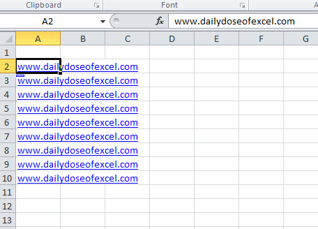
I say “seems like” because Excel only recognizes one. And to be even more precise, it recognizes pieces of both hyperlinks to make one. Let me explain. If I type a URL in a cell, Excel converts it into a hyperlink. (Pro Tip: Press Ctrl+Z immediately after the conversion to undo the conversion, but keep the text). Let’s say I copy that down a few cells.

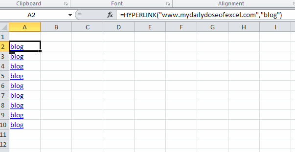
Now let’s say that I edit these cells to contain a HYPERLINK formula with a different address and a different display text. In this case, I’ve change the address by adding “my” in front of it and change the display text from the URL to the word “blog”.

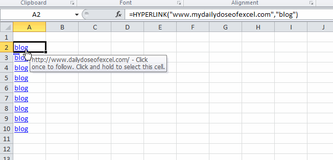
If I hover over the new hyperlink, check what happens. There are three important properties of hyperlinks: Address (where it goes when you click), Text to Display (what shows up in the cell), and Tooltip (what pops up when you hover). With two hyperlinks, it appears that the Address and tooltip are driven by the embedded hyperlink and the Text to Display is driven by the formula.

I don’t know why it happens this way. I can’t even come up with a good story about how it’s an unintended consequence of some design decisions on Microsoft’s part. But it is what it is. I don’t know of any quick way to fix this through the user interface, but I wrote a macro to fix it.

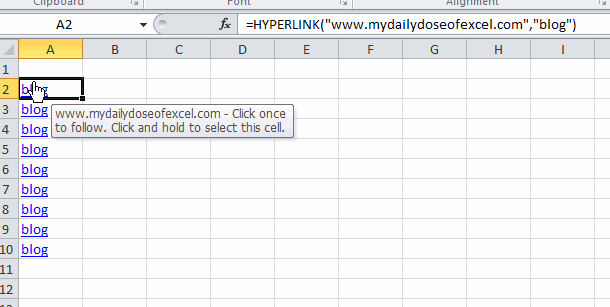
The code removes the embedded hyperlink and leaves the formula. The line that sets the formula equal to the formula is get the blue underline formatting back. The traditional hyperlink formatting disappears when you delete the hyperlink even though the formula remains. You can see that the tooltip now draws from the only remaining hyperlink, the formula one.