I started by showing you my awesome code to parse the SourceData of a pivot table. Code that has been rendered obsolete by John’s comment. I was going to continue with the supporting utilities used by the main procedure, but it may be hard to put things into context, so I’ll show the main procedure instead.
Dim rSource As Range
Dim vaFilters As Variant
Dim i As Long
Dim rFound As Range
Dim lField As Long
Dim lOldCalc As Long
Dim lFilterCnt As Long
Set rSource = Application.Evaluate(Application.ConvertFormula(pt.SourceData, xlR1C1, xlA1))
rSource.Parent.AutoFilterMode = False
lFilterCnt = FilterCount(Target)
If lFilterCnt > 0 Then
vaFilters = GetFilters(Target, lFilterCnt)
lOldCalc = Application.Calculation
Application.Calculation = xlCalculationManual
With rSource
.AutoFilter
For i = LBound(vaFilters, 1) To UBound(vaFilters, 1)
Set rFound = rSource.Rows(1).Find(vaFilters(i, 1), , xlValues, xlWhole)
If Not rFound Is Nothing Then
lField = rFound.Column – rSource.Cells(1).Column + 1
.AutoFilter lField, vaFilters(i, 2)
End If
Next i
End With
Application.Calculation = lOldCalc
End If
rSource.Parent.Activate
End Sub
I pass in two variables, Target and pt. Target is a variable in a DoubleClick event – the cell that was double clicked. The pt variable is the pivot table that contains that cell. I do all the testing for whether the cell is actually in a pivot table in the calling procedure, which I’ll show later. I could pass the Target and derive the pivot table via Set pt = Target.PivotTable, but since I already do it in the calling procedure, I don’t do it again.
The main idea of this code is to determine all the filters that are placed on the specific cell in the pivot table, then to create an autofilter on the source data with the same filters. For most cells in a pivot table, the filters applied can come from three places: The row it’s in, the column it’s in, and the page. Let’s look at an example.
Data like this
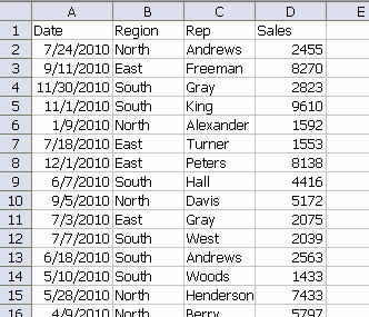
might produce a pivot table like this
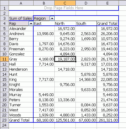
The cell that intersects Gray and North is affected by two filters, Rep and Region. My vaFilters Variant Array holds the filters that I will use to create the autofilter. It looks like this
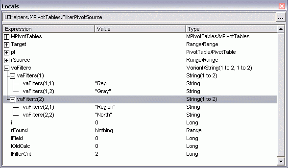
I’ll show the code that counts the filters and fills the array in a later post. Once I have the filters, I set calculation to manual. That cut the code processing time from almost three seconds to less than 1/2 second.
With the source range, I apply an AutoFilter. Then I loop through all my filters and find the column to which that filter relates. Assuming I found it, I set the AutoFilter constraint using the second value in my array. For instance, I search for the column in my source range with “Rep” in the first row. I compute where in the source range it is and store that in lField. Then I set the autofilter to “Gray”. On the second loop, I do the same thing for “Region” and “North”. With the data properly filtered, I activate the sheet that contains the data.
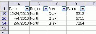
Currently this only works for Excel 2003. Excel 2007 introduces some wrinkles into the process that I haven’t attempted to iron out yet. There is also this pesky little problem of grouped dates. If my pivot table looks like this instead
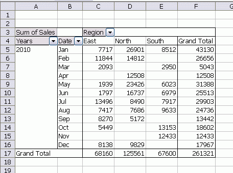
the grouped dates don’t play so nice. I’m working on that, but it’s not going well.
In my next post, I’ll show how I compute the number of filters and fill the array.
Posting code? Use <pre> tags for VBA and <code> tags for inline.