I’m wondering if this same Array -> Range approach will work with a non-contiguous range?
For example we have an application at work that needs to write around 400 values into an Excel sheet (it does this via ActiveXObjects from the browser. Yuck, I know). At present it does this in a loop calling .cell(row, column) and setting the value property.
I imagine doing Range(“A1, B10, C15, etc”).value = SOME ARRAY, would be much quicker but I’ve been hunting the web for a while now and haven’t found anyone who has done this. Perhaps it’s just not possible?
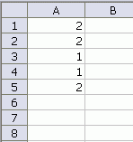
There is absolutely, positively no way this would work. Except that it does. I have this

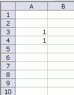
I want to write to A1, A2, and A5 without affecting A3 or A4.
Dim aWrite(1 To 5, 1 To 1) As Long
aWrite(1, 1) = 2
aWrite(2, 1) = 2
aWrite(5, 1) = 2
Union(Range(“A1:A2”), Range(“A5”)).Value = aWrite
End Sub
And I get this

It doesn’t matter if I fill aWrite(3,1) or aWrite(4,1). In this example I left them blank. But if I fill them, it still leaves A3:A4 untouched. I didn’t know you could do that.
Didn’t know that either… that’s a pretty cool trick.
I don’t think it actually works for arrays, though:
set r=union([q42],[z99])
r.value=[{42,99}]
typed at the Immediate window command line just puts 42 in both cells…
Actually, it does something not really desired. If we have different values in the array, as in the code below, the result shows a pattern that I cannot fathom.
Sub testnocon()
Dim aWrite(1 To 11, 1 To 1) As Long
aWrite(1, 1) = 2
aWrite(2, 1) = 3
aWrite(5, 1) = 4
aWrite(6, 1) = 5
aWrite(7, 1) = 6
aWrite(9, 1) = 7
aWrite(10, 1) = 8
aWrite(11, 1) = 9
Union(Range(“A1:A2”), Range(“A5:a7”), Range(“A9:a11”)).Value = aWrite
End Sub
The result is
2
3
2
2
2
2
3
0
Ooh, that’s nasty. I guess I was right the first time – not possible. :)
Oddly, this gives the same answer
Using Tushar’s setup, why not just read in the full range, change what you want and write it back out again?
Sub testnocon2()
Dim aWrite As Variant
aWrite = WorksheetFunction.Transpose(Range(“A1:A11?))
aWrite(1) = 2
aWrite(2) = 3
aWrite(5) = 4
aWrite(6) = 5
aWrite(7) = 6
aWrite(9) = 7
aWrite(10) = 8
aWrite(11) = 9
Range(“A1:A11?).Value = WorksheetFunction.Transpose(aWrite)
End Sub
Results are definitely unreliable. Rick’s approach makes sense, but personally I wouldn’t screw around transforming ranges. I’d just use a second array index, e.g., aWrite(2, 1) = 3.
Rick: The problem is if there are formulas in the range. I thought it would be cool to write a bunch of values and leave the formulas in tact.
I’m glad I started reading the comments before I started implementing this code! I had been looking for a solution like this but could find one. I guess I’ll still have to use my work around.
If the formulas aren’t array formulas wouldn’t this work?
dim r1 as range
dim v1 as variant
v1=r1.formula
@Dick,
Okay, then Transpose the formulas instead of the Values. You can then assign constants or other formulas to a smaller subset of the range and the original formulas will remain intact…
Sub testnocon2()
Dim aWrite As Variant
aWrite = WorksheetFunction.Transpose(Range(“A1:A11?).Formula)
aWrite(1) = “=SUM(D1:D4)”
aWrite(2) = “=IF(B1=””””,””Okay””,””Not Okay””)”
aWrite(5) = 1
aWrite(6) = 2
aWrite(7) = “=SUM(D5:D7)”
aWrite(9) = 3
aWrite(10) = “=IF(B1=””””,””Okay””,””Not Okay””)”
aWrite(11) = 4
Range(“A1:A11?).Formula = WorksheetFunction.Transpose(aWrite)
End Sub
Strange indeed. Entering:
[a1:c3,a5:c7,a9:c11,a13:c15]=[{1;2;3}+{0,10}]
from the immediate window shows that when assigning arrays to multi-area ranges the values in the 1st, 3rd, 5th,… areas are returned as if the formula were array-entered into each. However the values in the 2nd, 4th, 6th, … appear to be transposed and either wrap around in the case of multiple columns or repeat if only one single column is used. No idea what should cause this?
I understand it’s possible to write arrays to ranges more efficiently by calling the xlSet API function via a DLL but have not tried this in practice.
Rick – like fzzz I’m puzzled as to why you do the two transposes.
Not like you to use 28 key strokes when zero would do, so is there a reason?
I approached with
[A1:A10] = [IF(isblank(A1:A10),{22;33;44;55;66;77;88;99;10;11},A1:A10)]
End Sub
But this removes all the formulae
So I had to add:
sq = [A1:A10].Formula
[A1:A10] = [IF(isblank(A1:A10),{22;33;44;55;66;77;88;99;10;11},A1:A10)]
For j = 1 To UBound(sq)
If InStr(sq(j, 1), “=”) = 1 Then [A1:A10].Cells(j) = sq(j, 1)
Next
End Sub
I recently faced with a sort of this task – I needed to scroll through selected cells of a range (could be a filtered range) and multiply numbers to (-1). Cells with other data types are to remain untouched
After several attempts I found that two ranges are to be determined: Original non-continuious range (range A) and continious range (range B) that covers entirely range A. Range B is estimated from the boundaries of range A.
Array is bound to the range B
Tnen the code runs through each cell of range B and checks its intersction with range A. If so, array’s element is filled with the new estimated value. If not arrays’s element inherits original untouched value
That it is the basic logic and it works well. The code is enclosed (sorry it is a bit bulky)
‘
Dim rngRange As Range ‘Initial discontinious range
Dim rngRangeContinious As Range ‘Final continious range
Dim lng1stRow As Long ‘First Row number (of potential continious range)
Dim byt1stCol As Byte ‘First Column number (of potential continious range)
Dim lngLastRow As Long ‘Last Row number (of potential continious range)
Dim bytLastCol As Byte ‘Last Column number (of potential continious range)
Dim rngArea As Range ‘Range-segment(s) in initial discontinious range
Dim intAreaCounter As Integer ‘Counter of range-segments
Dim lngRows As Long ‘Number of rows in final continious range
Dim bytCols As Byte ‘Number of columns in final continious range
Dim lngRow As Long ‘Number of rows in array
Dim bytCol As Byte ‘Number of columns in array
Dim avarValues() As Variant ‘Array (initially with no dimensions; for data of any type)
Dim rngIntersection As Range ‘Intersection (cell of Final continious range with initial range)
Dim varValue As Variant ‘Converted value (of any type) written to array
On Error GoTo ErrorHandler ‘ Enable error-handling routine
‘Turning off screen updates (speed increasing)
With Application
.EnableEvents = False
.ScreenUpdating = False
End With
‘Visible cells selection (useful for filtered ranges)
If Application.Union(Selection, Selection).Count > 1 Then Selection.SpecialCells(xlCellTypeVisible).Select
‘Shortened range – double selections are omitted
Set rngRange = Application.Union(Selection, Selection)
‘Cycle check in all discontinious areas of the selection
For Each rngArea In rngRange.Areas
With rngArea
‘First Row
If lng1stRow = 0 Or lng1stRow > .Row Then
lng1stRow = .Row
End If
‘Last Row
If lngLastRow <= .Row + .Rows.Count – 1 Then
lngLastRow = .Row + .Rows.Count – 1
End If
‘First column
If byt1stCol = 0 Or byt1stCol > .Column Then
byt1stCol = .Column
End If
‘Last Column
If bytLastCol <= .Column + .Columns.Count – 1 Then
bytLastCol = .Column + .Columns.Count – 1
End If
intAreaCounter = intAreaCounter + 1
End With
Next rngArea
‘Whole range that covers all discontinious ones
Set rngRangeContinious = Range(Cells(lng1stRow, byt1stCol), Cells(lngLastRow, bytLastCol))
‘Counting of rows for array
With rngRangeContinious
lngRows = .Rows.Count
bytCols = .Columns.Count
End With
‘Sizing of array
ReDim avarValues(1 To lngRows, 1 To bytCols)
‘Filling of array
For lngRow = 1 To lngRows
For bytCol = 1 To bytCols
‘Intersection check
Set rngIntersection = Application.Intersect(Cells(lng1stRow + lngRow – 1, byt1stCol + bytCol – 1), rngRange)
If rngIntersection Is Nothing Then ‘Cell is out of initial range then it remains unchanged
varValue = Cells(lng1stRow + lngRow – 1, byt1stCol + bytCol – 1).Value
Else
‘Validation of values
Select Case VarType(Cells(lng1stRow + lngRow – 1, byt1stCol + bytCol – 1).Value)
Case 1 To 6 ‘Numbers
varValue = Cells(lng1stRow + lngRow – 1, byt1stCol + bytCol – 1).Value * (-1)
Case Else ‘Others
varValue = Cells(lng1stRow + lngRow – 1, byt1stCol + bytCol – 1).Value
End Select
End If
‘Filling of element of array
avarValues(lngRow, bytCol) = varValue
Next bytCol
Next lngRow
‘Filling the selection from array
‘Important Check! Is AutoFilter is working or not!
‘If it is working then array elements are inserted into the range
‘incorrectly (1st element only). So the filter has to be temporarily
‘deactivated and then restored
If Worksheets(ActiveSheet.Name).FilterMode = True Then ‘Filter is working
‘ ===
‘oine workaround created and then disabled
‘reason – too slow performance of CustomViews.Show action :(
‘ With ActiveWorkbook
‘ .CustomViews.Add ViewName:=”TempView”, PrintSettings:=False, _
‘ RowColSettings:=True ‘Temporary Custom View is created
‘ Worksheets(ActiveSheet.Name).AutoFilterMode = False ‘AutoFilter is off
‘ rngRangeContinious = avarValues ‘Range filling from array
‘ .CustomViews(“TempView”).Show ‘Custom View is applied
‘ .CustomViews(“TempView”).Delete ‘Custom View is deleted
‘ End With
‘ ===
Dim wshWorksheet As Worksheet
Dim rngFilterRangeAddress As String
Dim bytFilterNumber As Byte
Dim bytColumn As Byte
Dim filterArray()
Set wshWorksheet = Worksheets(ActiveSheet.Name) ‘Name of current sheet
With wshWorksheet.AutoFilter
rngFilterRangeAddress = .Range.Address ‘Filtered range
With .Filters
ReDim filterArray(1 To .Count, 1 To 3) ‘Filter Array
For bytFilterNumber = 1 To .Count
With .Item(bytFilterNumber)
If .On Then
filterArray(bytFilterNumber, 1) = .Criteria1
Select Case .Operator ‘Check for presence of Operator or criteria2
Case 3 To 6 ‘Top selection
Case Empty ‘No second criteria
Case Else ‘Two criteria are selected
filterArray(bytFilterNumber, 2) = .Operator
filterArray(bytFilterNumber, 3) = .Criteria2
End Select
End If
End With
Next
End With
End With
wshWorksheet.AutoFilterMode = False ‘Turn off autofilter
rngRangeContinious = avarValues ‘Range filling from array
For bytColumn = 1 To UBound(filterArray(), 1) ‘Restore
If Not IsEmpty(filterArray(bytColumn, 1)) Then
If filterArray(bytColumn, 2) Then
wshWorksheet.Range(rngFilterRangeAddress).AutoFilter field:=bytColumn, _
Criteria1:=filterArray(bytColumn, 1), _
Operator:=filterArray(bytColumn, 2), _
Criteria2:=filterArray(bytColumn, 3)
Else
wshWorksheet.Range(rngFilterRangeAddress).AutoFilter field:=bytColumn, _
Criteria1:=filterArray(bytColumn, 1)
End If
End If
Next
Else
rngRangeContinious = avarValues ‘Range filling from array
End If
”
‘Turning on screen updates
With Application
.EnableEvents = True
.ScreenUpdating = True
End With
‘Error-handling routine
ErrorHandler:
If Err.Number = 1004 Then ‘Evaluate error number 1004
MsgBox “Excel standard error # “ & Err.Number & “:” & vbCr & vbCr & Err.Description & _
vbCr & “============================OR==============================” & _
vbCr & Chr(5) & ” Try to select less rows in a filtered range.”, vbCritical, “Too many filtered rows”
End If
End Sub
Ivan,
Why couldn’t you just enter the -1 in a random cell, copy it, then paste special multiply to visible cells only?
@Ivan,
I would agree with zach and do it using Paste Special (Multiply); however, if you found that you did need to use code to perform this action, I believe this much short macro would do the job for you…
Sub Cells_To_Minus_And_Vise_Versa()
Dim Cell As Range
For Each Cell In Selection.SpecialCells(xlCellTypeVisible).SpecialCells(xlCellTypeConstants, xlNumbers)
Cell.Value = -1 * Cell.Value
Next
End Sub
Note: I left out the error-checking code which you could provide if you think there will be more than 8192 discontiguous areas (areas being ranges of contiguous cells) which is a limit for SpecialCells in versions of Excel before XL2010.
Gentlemen,
An idea with PasteSpecial/Multiply did not come to my mind. You are probably right and it is worth testing on big numbers of ranges (especially when AutoFilter is on)
Regarding ‘For Each Cell’ construction – I had created more or less similar code long ago (here it is)
‘ Macro recorded 26/06/2003’
Dim rngCell As Range
Selection.SpecialCells(xlCellTypeVisible).Select
For Each cell In Selection
Select Case VarType(cell.Value)
Case 1 To 6
cell.Value = cell.Value * (-1)
End Select
Next
End Sub
The practice showed that this code works rather slowly on big numbers of non-contiguous ranges. Sometimes it took minutes to run through all the cells and update them
That is why I had to use another approach with arrays and succeeded in end-user performance. The code works with steady speed for any number of ranges
Besides my particular example is a relative one. Just to demonstrate a way of filling of non-contiguous ranges through array