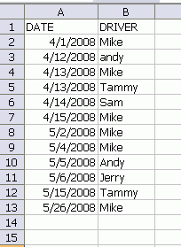
and she wants to know who used the vehicle the most by month. I couldn’t think of an easy way to do this with worksheet functions, so I resorted to a pivot table.
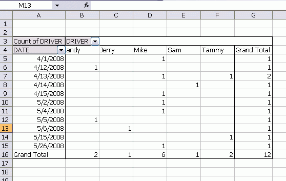
With Date on the left, Driver across the top, and Count of Driver in the data area, I grouped the date on month (right click – group and show detail – group).

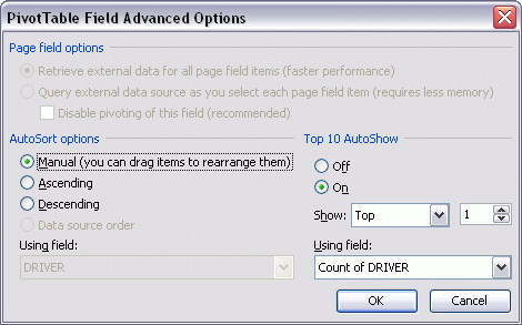
Finally, I went to Field Settings for the Driver field (the one across the top) and showed the Top 1
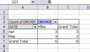
I went back to the data and changed a few ‘Mikes’ to ‘Tammys’ in May and here’s what that looks like. With a sufficiently large data set, it seems like showing Top 1 wouldn’t make any difference because it would just show all the columns anyway.
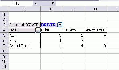
Better ways to get this data?
I would have used conditionnal formatting in the pivot table.
Not that good because pivot table expand and collapse easily, but this would be the fastest way.
Alternative: month 4 in column J, month 5 in column 5
[J2:J13] = [if(month(A2:A13)=4,B2:B13,“”)]
[J2:J13] = [if(J2:J13<>“”,countif($J$2:$J$13,J2:J13) & ” “ &J2:J13,“”)]
[J2:J13] = [if(countif(offset($J$2,,,Row(2:13)-1),J2:J13)=1,J2:J13,“”)]
[J2:J13].Sort [J2], xlDescending
[K2:K13] = [if(month(A2:A13)=5,B2:B13,“”)]
[K2:K13] = [if(K2:K13<>“”,countif($K$2:$K$13,K2:K13) & ” “ &K2:K13,“”)]
[K2:K13] = [if(countif(offset($K$2,,,Row(2:13)-1),K2:K13)=1,K2:K13,“”)]
[K2:L13].Sort [K2], xlDescending
End Sub
I would probably just Pivot it too. The only difference is that I would use DRIVER as the Row Label, and then COUNT OF DATE in the Values area.
Here’s another way with worksheet formulas.
1. Figure out all of the unique names in the list. Do this by choosing Data > Filter > Advanced Filter. Choose “Copy to another location” and check “Unique records only”.
2. Next to the filtered list of names (suppose they start in D2), enter the following formula in E2 and then fill down:
=COUNTIF($B$2:$B$13,”=”&D2)
That will be equivalent to evaluating
E2 =COUNTIF($B$2:$B$13,”=Andy”)
E3 =COUNTIF($B$2:$B$13,”=Jerry”)
etc.
The comparison will treat both “andy” and “Andy” as the same; i.e. it is not case sensitive. But an extra trailing space will cause trouble. E.g. if the cell’s text is really “Andy “, then Andy-space will look a different entry from “Andy”.
Oh, and then I would sort descending on column E!
This is my first time posting here so I hope this actually works.
I have accomplished this using first the Max(if) array formula, then nested offset and nested match functions.
[is there a way to post screen shots in comments? do i need to upload the pic somewhere else first?]
I added more data to Tammy’s original some dates for Jan & Feb. The results, using a Sum array formula, is this for each person: (Table A)
12345
Mike21035
Andy30010
Tammy04010
Sam00010
Jerry11001
(the top row are the # values for the month).
Now, to match the max for each month to the person who acheived it.
Table B- these are my results. Column 3 produces the name using excel functions
Month #Max #Name
13Andy
24Tammy
30Mike
43Mike
55Mike
The first column are the month values again. The second column uses this Max array formula to find the max: {=MAX(IF($F$1:$J$1=$E10,$F$2:$J$6))}
The third column uses Match to first find the correct column in Table A for the month from column 1 in Table B; then Match (along with the offset for the # I just got) to identify which row of Table A the max value from Column 2 Table B is in. Finally, those 2 numbers give the parameters by which to identify the name using the Index function.
=OFFSET($E$1,MATCH($F10,OFFSET($E$2:$E$6,,MATCH($E10,$F$1:$J$1,0),,),0),,,)
[…] Most Frequent Occurence […]
This was the fastest way I could do it using just workbook functions (trying to avoid the pivot table). This gets the job done in a few minutes.
Enter formula in C3: =MONTH(A2)
Drag C3 down
Enter headings on D2 and E2 of April and May
Enter formula in D2: =COUNTIFS($C$2:$C$13,”4?,$B$2:$B$13,$B2)
Drag D2 down
Enter formula in D14: =INDEX($B2:$B13,MATCH(MAX(D2:D13),D2:D13,0),1)
Drag D2:D14 over
I should add that I know that one problem with my solution above is that if more than one item has the max value, it will only return the first one it finds in the summary table for each month. (so, the first name in the list). for instance, the 3rd month gave Mike’s name even though he had zero.
But that was not listed as part of the question. It seems that it would take VBA and multiple cells to pull off multiple max’s.
@Dick
Wrong pivot Layout…..
See this
http://tinypic.com/r/23h4lyw/6
The Top 1 will then work correctly
Pivot is probably better here, but perhaps also try with ctrl+shift+enter:
=INDEX(Driver,MODE(IF(TEXT(Date,”yyyy-mm-1″)=D2,MATCH(Driver,Driver,0))))
where D2=month (eg May-08), Date=a2:a13, Driver=b2:b13.
The new MODE.MULT function could be put to use for the multiple driver case maybe?
The Duplicate Master addin will also do this, , http://www.experts-exchange.com/A_2123.html
Normally I’d also use a PivotTable, but if case sensitivity, white spaces, or mis-spelt strings need matching then the addin provides flexibility to cater for this
Cheers
Dave
A tabulated result using Ihm’s formula
D2: =A2-DAY(A2)+1
D3: =IF(ISERROR(MATCH(0,COUNTIF(D$2:D2,($A$2:$A$20-DAY($A$2:$A$20)+1)&””),0)),””,
INDEX(IF(ISBLANK($A$2:$A$20),””,$A$2:$A$20-DAY($A$2:$A$20)+1),MATCH(0,COUNTIF(D$2:D2,($A$2:$A$20-DAY($A$2:$A$20)+1)&””),0)))
D3 is an array formula, copy down as far as you need
E2: =INDEX(Driver,MODE(IF(date-DAY(date)+1=D2,MATCH(Driver,Driver,0))))
also an array formula, copy down as far as Column D goes