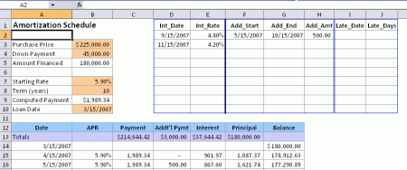
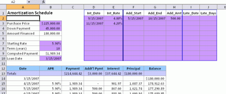
Here’s a utility to format unlocked cells using conditional formatting so that I can easily see that I’ve set the Locked property appropriately.
Sub ToggleLockedCellFormat()
Dim sh As Worksheet
Dim rng As Range
Dim fc As FormatCondition
Dim lFcIndex As Long
Set sh = ActiveSheet
Set rng = sh.UsedRange
rng.Cells(1).Select
msFormula = “=NOT(CELL(““protect”“,” & rng.Cells(1).Address(0, 0) & “))”
If sh.ProtectContents Then
MsgBox “You can’t use this on a protected sheet.”
Else
If rng.FormatConditions.Count = -1 Then
‘-1 means that not all cells have the same conditional formatting
MsgBox “You can’t use this when conditional formatting is present.”
Else
If LockedShown(rng, lFcIndex) Then
‘lFcIndex will hold the number of the format condition
‘that has the right formula – the one to delete.
rng.FormatConditions(lFcIndex).Delete
Else
Set fc = rng.FormatConditions.Add(xlExpression, , msFormula)
fc.Interior.Color = RGB(204, 153, 255)
‘ugly purple that would never be used in a real spreadsheet
End If
End If
End If
End Sub
Private Function LockedShown(rng As Range, ByRef lFcIndex As Long) As Boolean
Dim i As Long
Dim bReturn As Boolean
bReturn = False
For i = 1 To rng.FormatConditions.Count
If rng.FormatConditions(i).Formula1 = msFormula Then
lFcIndex = i
bReturn = True
Exit For
End If
Next i
LockedShown = bReturn
End Function
It won’t work on a protected sheet or if there is conditional formatting already on the sheet. Well, that’s not entirely true. If there is conditional formatting that covers the whole used range, it will work. It only doesn’t work if the conditional formatting that’s present isn’t consistent across all cells in the used range.
Before

After

I haven’t tested it in 2007 or 2010, but if you’d like to, leave a comment.
Here is a non-coded method to identify the unlocked cells that you and your readers might like to try. Go to the sheet you want to test and select Edit/Find from the menu bar. If all the Options are not displayed, click the “Options>>” button to display them. First off, clear the “Find what” field so that it is empty. Next, click the “Format…” button, then click the “Protection” tab on the dialog box that was displayed. Then click the “Locked” and “Hidden” checkboxes (as much as needed) until they are both completely clear (not checked and not grayed out) and click the “OK” button. Finally, click the “Find All” button, then press Ctrl+A on the keyboard and then click the “Close” button. All the unlocked cells should now be selected.
Nice to see some alternatives.
As I am stuck in Excel 2003, I always follow the same process – which is:
Save the current file.
Save a copy as xxxx_Test
Run check macro against it
This identifies all the unlocked cells in every worksheet by adding in a pattern, so that they are immediately obvious.
Works a treat if you have colour coded cells, as it leaves the base colour as it was.
Just a follow up to my last message… if you want to do the selection process I outlined in my previous message using code (attached to a button perhaps?), then here is a macro you could use to do that…
Dim FirstAddress As String, C As Range, U As Range
Application.FindFormat.Locked = False
Set C = ActiveSheet.UsedRange.Find(“”, SearchFormat:=True)
If Not C Is Nothing Then
FirstAddress = C.Address
Do
If U Is Nothing Then
Set U = C
Else
Set U = Union(U, C)
End If
Set C = ActiveSheet.UsedRange.Find(“”, After:=C, SearchFormat:=True)
Loop While Not C Is Nothing And C.Address <> FirstAddress
U.Select
End If
End Sub
Okay, this was a fun exercise to do! Below is a stand-alone macro (no side function needed) which appears to do what your macro does (toggles the conditionally format interior color for the unlocked cells on and off using that ugly purple color for the “on” condition). The only drawback I can see with my macro is if the number of unlocked cells is very large (the Union method will get progressively slower as the number of elements in the union goes up); however, if the number of unlocked cells is not very large, then my macro has the advantage that it only iterates the unlocked cells rather than every cell in the UsedRange. Anyway, for what it is worth, here is my toggle macro…
Dim MaxFC As Long, FirstAddress As String, HighliteColor As Long
Dim FC As FormatCondition, C As Range, U As Range
Const CFformula As String = “=NOT(CELL(““protect”“))”
HighliteColor = RGB(204, 153, 255)
Application.FindFormat.Locked = False
Set C = ActiveSheet.UsedRange.Find(“”, SearchFormat:=True)
If Not C Is Nothing Then
FirstAddress = C.Address
Do
If U Is Nothing Then
Set U = C
Else
Set U = Union(U, C)
End If
Set C = ActiveSheet.UsedRange.Find(“”, After:=C, SearchFormat:=True)
Loop While Not C Is Nothing And C.Address <> FirstAddress
U(1).Select
MaxFC = U.FormatConditions.Count
If MaxFC = -1 Or MaxFC = 3 Then
MsgBox “You can’t use this when conditional formatting is present.”
Else
If MaxFC > 0 Then
If U.FormatConditions(MaxFC).Interior.Color = HighliteColor Then
U.FormatConditions(MaxFC).Delete
Else
Set FC = U.FormatConditions.Add(xlExpression, , CFformula)
FC.Interior.Color = RGB(204, 153, 255)
End If
Else
Set FC = U.FormatConditions.Add(xlExpression, , CFformula)
FC.Interior.Color = RGB(204, 153, 255)
End If
End If
End If
End Sub
One more tweak…
This version preserves the active cell location (wherever it is when you call the macro is where it will be after the macro finishes toggling the display)…
Dim HighliteColor As Long, MaxFC As Long, FC As FormatCondition
Dim FirstAddress As String, CurrentCell As String, C As Range, U As Range
Const CFformula As String = “=NOT(CELL(““protect”“))”
HighliteColor = RGB(204, 153, 255)
Application.FindFormat.Locked = False
Set C = ActiveSheet.UsedRange.Find(“”, SearchFormat:=True)
If Not C Is Nothing Then
FirstAddress = C.Address
Do
If U Is Nothing Then
Set U = C
Else
Set U = Union(U, C)
End If
Set C = ActiveSheet.UsedRange.Find(“”, After:=C, SearchFormat:=True)
Loop While Not C Is Nothing And C.Address <> FirstAddress
CurrentCell = ActiveCell.Address
U(1).Select
MaxFC = U.FormatConditions.Count
If MaxFC = -1 Or MaxFC = 3 Then
MsgBox “You can’t use this when conditional formatting is present.”
Else
If MaxFC > 0 Then
If U.FormatConditions(MaxFC).Interior.Color = HighliteColor Then
U.FormatConditions(MaxFC).Delete
Else
Set FC = U.FormatConditions.Add(xlExpression, , CFformula)
FC.Interior.Color = RGB(204, 153, 255)
End If
Else
Set FC = U.FormatConditions.Add(xlExpression, , CFformula)
FC.Interior.Color = RGB(204, 153, 255)
End If
End If
Range(CurrentCell).Select
End If
End Sub
In my “one more tweak” message, I accidentally used the wrong macro name (not a big deal as far as execution goes, of course, but it might be confusing as to intent)… the macro should have been named ToggleUnlockedCellsColor, not SelectUnlockedCells (which was the correct name for the macro in my second message in this thread only). Sorry for the confusion for anyone actually reading my comments.[grin]
What would be wrong with:
If cel.Locked Then
If rngLocked Is Nothing Then
Set rngLocked = cel
Else
Set rngLocked = Union(rngLocked, cel)
End If
End If
Next cel
Uses selection instead of conditional format.
Oops…. I forgot:
@Alex,
If your question was directed at me, then the reason behind my code is I did not want to test every cell in the used range for what I assume would be not all that many unlocked cells (think 10,000 cells in the used range with only 500 of them unlocked).
@Rick,
Actually, no, the find mechanism is really cool. I wanted to use Select instead of colour to identify the locked cells, and I hadn’t yet figured out how to get the Find method to select-all.
@AlexJ,
Did you see my second message in this thread (the one where I first posted some code)? That macro uses my Find method to **select** (not color) the unlocked cells. I later changed it to become a color toggle in my follow up messages, but the first code I posted does what you are talking about.
I like the CF rather than selecting so I can go lock/unlock the cells I screwed up and still see the pattern.
@Rick,
Quite right – I missed the first post – I was so dazzled with the conditional formatting code! :-)
Another approach is to introduce a deliberate error to a replica worksheet and then use SpecialCells to quickly return the unlocked cell range – no looping required
Dim ws1 As Worksheet
Dim ws2 As Worksheet
Dim rng1 As Range
Dim rng2 As Range
Dim rng3 As Range
Dim lCalc As Long
Dim bWorkbookProtected
On Error Resume Next
‘test to see if WorkBook structure is protected
‘if so try to unlock it
If ActiveWorkbook.ProtectStructure Then
ActiveWorkbook.Unprotect
If ActiveWorkbook.ProtectStructure Then
MsgBox “Sorry, I could not remove the passsword protection from the workbook” _
& vbNewLine & “Please remove it before running the code again”, vbCritical
Exit Sub
Else
bWorkbookProtected = True
End If
End If
Set ws1 = ActiveSheet
‘test to see if current sheet is protected
‘if so try to unlock it
If ws1.ProtectContents Then
ws1.Unprotect
If ws1.ProtectContents Then
MsgBox “Sorry, I could not remove the passsword protection from sheet” & vbNewLine & ws1.Name _
& vbNewLine & “Please remove it before running the code again”, vbCritical
Exit Sub
End If
End If
On Error GoTo 0
‘disable screenupdating, event code and warning messages.
‘set calculation to manual
With Application
.ScreenUpdating = False
.EnableEvents = False
.DisplayAlerts = False
lCalc = .Calculation
.Calculation = xlCalculationManual
End With
On Error Resume Next
‘check for existing error cells
Set rng1 = ws1.Cells.SpecialCells(xlCellTypeFormulas, 16)
On Error GoTo 0
‘copy the activesheet to a new working sheet
ws1.Copy After:=Sheets(Sheets.Count)
Set ws2 = ActiveSheet
‘delete any cells that already contain errors
If Not rng1 Is Nothing Then ws2.Range(rng1.Address).ClearContents
‘protect the new sheet
ws2.Protect
‘add an error formula to all unlocked cells in the used range
‘then use SpecialCells to read the unlocked range address
On Error Resume Next
ws2.UsedRange.Formula = “=NA()”
ws2.Unprotect
Set rng2 = ws2.Cells.SpecialCells(xlCellTypeFormulas, 16)
Set rng3 = ws1.Range(rng2.Address)
ws2.Delete
On Error GoTo 0
‘if WorkBook level protection was removed then reinstall it
If bWorkbookProtected Then ActiveWorkbook.Protect
‘cleanup user interface and settings
With Application
.ScreenUpdating = True
.EnableEvents = True
.DisplayAlerts = True
lCalc = .Calculation
End With
‘inform the user of the unlocked cell range
If Not rng3 Is Nothing Then
MsgBox “The unlocked cell range in Sheet “ & vbNewLine & ws1.Name & ” is “ & vbNewLine & rng3.Address(0, 0)
Else
MsgBox “No unlocked cells exist in “ & ws1.Name
End If
End Sub
Very nice! You can also do this with conditional formatting.
http://densom.blogspot.com/2011/08/highlight-protected-cells-in-excel.html
– Dennis
I had another idea for this. If there is no coloring on the sheet (either interior or conditional formatting), then perhaps this somewhat short macro that toggles locked cell’s interior color might be useful…
Static InteriorColor As Long
If InteriorColor = 0 Then InteriorColor = RGB(255, 255, 255)
InteriorColor = RGB(204, 153, 255) + RGB(255, 255, 255) – InteriorColor
Application.FindFormat.Locked = True
Application.ReplaceFormat.Interior.Color = InteriorColor
Cells.Replace “”, “”, , , , , True, True
End Sub