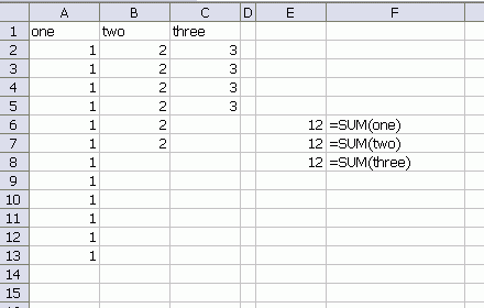
I had an occasion to create about 25 dynamic named ranges. A tedious process, that. So I cooked up some code. All the ranges needed to start in row 2 and extend down as far as there is data. There wouldn’t be any blanks, so I didn’t worry about it.

In this example, I select A1:C1 and run the code
Dim rCell As Range
Dim wb As Workbook, ws As Worksheet
Set ws = Selection.Parent
Set wb = ws.Parent
For Each rCell In Selection.Cells
wb.Names.Add rCell.Value, “=” & ws.Cells(2, rCell.Column).Address & _
“:INDEX(“ & rCell.EntireColumn.Address & _
“,COUNTA(“ & rCell.EntireColumn.Address & “))”
Next rCell
End Sub

Ah, but there’s a problem. I’m going to be using these named ranges in array formulas (or possibly SUMIFs). I need all these ranges to be the same number of rows. Since column A will never be blank, I’m going to use that as my row count anchor. I changed the code thusly:
“:INDEX(“ & rCell.EntireColumn.Address & _
“,COUNTA(“ & ws.Columns(1).Address & “))”
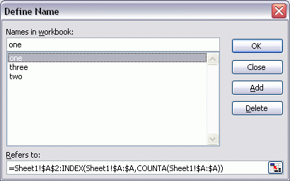
Now, for instance, the named range ‘three’ refers to
Since all the formulas COUNTA on column A, they’ll all be the same length. It’s not exactly error-proof or general-purpose, but it saved me some work today.
Create the column A name. Then for the remaining names use =offset(colAName,0,{n})
This way if you ever change the rule for what to include in col. A all the other names will change w/o any work on your part.
For me this was already part of the Name Manager on the HomeTab :-)
http://tinypic.com/view.php?pic=30j5qq9&s=5
I’ve recently started using MATCH instead of COUNTA in such expressions, to guard against the possibility that there are blank cells interspersed in the column. That makes the expression
=Sheet1!$A$2:INDEX(Sheet1!$A:$A,MATCH(10^200,Sheet1!$A:$A),1)
if the “last” value is expected to be a number, or
=Sheet1!$A$2:INDEX(Sheet1!$A:$A,MATCH(“ZZZZZZZZZZZ”,Sheet1!$A:$A),1)
if the “last” value is expected to be text.
Granted, having those blank cells is usually a mistake, but we all know what can happen once end users get a hold of our workbooks :)
Patrick,
You don’t need “zzzz..” you can use = Match(“*”,A:A,-1)
Sam, did you test that? eg =MATCH(“*”,CHAR(ROW(1:255)),-1) with ctrl+shift+enter returns #N/A.
You need to be careful with text comparisons, MS Office seems to follow closely this standard:
http://en.wikipedia.org/wiki/European_ordering_rules
An alternative to “*” is “” which would work if the range doesn’t contain empty strings. Also instead of “zzzz…” you could use a greek character like “a” but neither will allow for other unicode characters.
Running this from the debug window… for i=1 to 65535:cells(i,1)=chrw(i):next i
and sorting descending shows the level 1 sort order. The last is “?” U+3005 (12293) which could also be used with MATCH. Lori
Hi Dick
I created a Tutorial and an example file to do this same thing some while ago.
It can be found on Debra’s site
http://www.contextures.com/xlNames03.html
Cheers
Roger
My approach (when I used to interview Excel “developers” this was a favourite interview question) was identical to Tushtar’s. I suppose I’m an OFFSET() sort of guy. Also, I hadn’t ever considered that the result of an INDEX() might be useable as shown, so I learned something. I’d like to see if anyone can show which, if any, might be qualitatively better.
@Mike, most of the time, INDEX vs OFFSET probably makes no difference in terms of performance. I just try to stay away from OFFSET when I can because I try to minimize use of volatile functions.
But Sam…who uses Excel 2007 ?
Use Tables in Excel 2007. The bounds of the table are then known.
@Rob – Tables are not truly dynamic.
Try this
a) Create a table
b) Leave a couple of rows blank and paste some data
c) delete the blank rows
d) the Table does not expand automatically
Hi Sam
Once you have left blank rows, before entering more data, you are not entering data to the table.
The table object has terminated at the last row of data.
The only way of then incorporating the new rows of data, after deleting your blank entries is Design tab>Resize.
If you want blank rows within a table (which rather defeats the object of a table), then enter blank cells in the same way as you would input any data, and the table dimensions will adjust accordingly.
I don’t consider this a fair criticism of the dynamic property of Tables.
Hi Roger.
I know its a bit harsh… I just feel the table should auto expand without having to resize.
A Dynamic name does
Data = $A$1:Index($1:$65535,Counta($A:$A),Counta($1:$1)) or other variants of this will expand if the blank rows get deleted.
Sam: The problem with a dynamic named range is that a blank cell in the first column will upset the range boundaries.
I see silly workarounds like matching a very large number, or matching an asterisk, or calling a VB function to find the last row.
Much safer to define a colour scheme for a table, and use that.
@Rob
What’s wrong with using a UDF in the definition of a named range ?
To define a (column) range with header ‘heading 12’ in sheet1:
=INDIRECT(“Sheet1!”&Persnlk.xls!A_column(“Sheet1?;MATCH(“heading 12?;Sheet1!$1:$1;0)))
A_column = Sheets(c0).Cells(1, x).Resize(Sheets(c0).Cells(Rows.Count, x).End(xlUp).Row).Address
End Function