MaryAnn asks an interesting question.
In column A there is text that may or may not contain the name of a US state. In column B there is a list of US states. In column C, we want the column A text without the state names. I think this would be a pretty trivial piece of VBA, but I wanted to see if I could do it in a formula. Here’s what I came up with:
Got that? OK, maybe a little explanation is in order. As usual, I will explain from the inside out. Let’s start with this little nugget
Normally with FIND, you pass a find_text argument and a within_text argument and you get a number showing the position of find_text within within_text, like =FIND("Kus","Dick Kusleika") would return 6 because the find_text “Kus” first appears in the 6th position of within_text. If find_text is nowhere to be found in within_text, you get an error. What I’ve done above is pass an array of find_text’s and checked to see if any of the states exist in A1. The result of this is a 56 element array that kind of looks like this {TRUE;TRUE;TRUE....TRUE}. If there is no state name, all 56 elements will be TRUE. If there is a state name, at least one of the elements will be FALSE. That brings me to
MATCH returns the position of the first argument in the list (the list is the second argument). This MATCH function is looking for FALSE in the 56 element array described above. If it finds a FALSE in the list, it returns the position in the list of the first one it finds. If A1 is “Chairs Idaho”, the MATCH function will return 15 because Idaho is the 15th name in the list in column B. MATCH will return an error if there are no FALSE elements in the list, so I have to use the old IF(ISNA trick
I set the TRUE condition to 0. Since there are no state names if ISNA is true, I don’t really care what position it returns. Now that I know the position of the state in the list, I can return the state name with INDEX
I substitute and empty string for the state name
And TRIM the whole thing to remove leading and trailing spaces.
Dick –
Interesting post! Thank you for sharing.
I have two questions:
1. For my edification (because my VBA is very limited), would you do this same task in VBA? If it’s a lot of code, feel free to disregard this question.
2. As a whole, your formula worked perfectly. When I tried to drill down to the individual pieces (following your analysis), though, I got stuck:
=FIND($B$1:$B$5,A1) evaluates to #VALUE in all cases
=ISERR(FIND($B$1:$B$5,A1)) therefore always evaluates to TRUE. (Not desirable, under the circumstances.)
Can you explain what it is about =MATCH(FALSE,ISERR(FIND($B$1:$B$5,A1)),FALSE) that makes the inner FIND function correctly handle the array?
Regards,
Michael
And of course that should read “… [how] would you do this same task in VBA?”
@Dick…
It looks like if you move your entire list down one row and leave A1 empty, then this slightly shorter formula appears to work…
=TRIM(SUBSTITUTE(A1,INDEX(B$1:B$57,SUMPRODUCT(ROW(B$1:B$57)*ISNUMBER(SEARCH(B$1:B$57,A1)))-1),””))
I’m sorry, leave B1 empty (not A1).
For fun, here’s what I arrived at (array-entered):
=TRIM(SUBSTITUTE(A1,INDEX($B$1:$B$56,MAX(IF(ISNUMBER(MATCH(“*”&$B$1:$B$56&”*”,A1,0)),ROW($B$1:$B$56)))),””))
Of course the big caveat is that there is no more than 1 U.S. state/territory per cell in col. A.
Dick,
Thank you for the nice post
To work all formula must be matrix validated (CTRL+Uppercase+Enter)
Best regards
Jean Paul
Michael
The following User Defined Function will produce the same results
(Fingers crossed this comment box presents it correctly)
Function RemoveState(StatesRange As Range, TargetString As String) As String
Dim rng As Range, str As String
str = TargetString
For Each rng In StatesRange
If InStr(1, str, rng.Value) <> 0 Then
str = Trim(Replace(str, rng.Value, “”))
Exit For
End If
Next
RemoveState = str
End Function
Nice work, Dick!
One question: What will the result be if the string contains two states like “Chairs Florida New York”?
@Jean Paul… The formula I posted does **not** require you to commit it using Ctrl+Shift+Enter… the formula works fine just using Enter by itself to commit it.
Wasn’t this covered way back in David Hager’s Excel newsletter?
Make the ‘state’ list include D.C. as well as a blank row below Wyoming, so 52 rows in all. Then enter the following array formula in C1.
=SUBSTITUTE(A1,INDEX($B$1:$B$52,MATCH(1,COUNTIF(A1,”*”&$B$1:$B$52&”*”),0)),””)
Augmenting lists usually eliminates the need for space- and recalc time-wasting redundant expressions.
@fzz… Yes, that seems to work although you need to encase it within a TRIM function call to get rid of possible multiple internal and/or trailing spaces.
Micheal, Jean Paul: Mine are array formulas, entered with ctl+shift+enter. See
http://www.dailydoseofexcel.com/archives/2004/04/05/anatomy-of-an-array-formula/
When I was writing this post, I was going to point to that post for anyone who doesn’t know what an array formula is. When I got there, I learned that my new CodeColerer add-in was screwing up code tags with no arguments (or so I thought) and that post was a mess. By the time I fixed it all up (with JP’s help), I’d forgot about creating the link.
David: It will only do the first state.
Yeah, I forgot the TRIM.
Another alternative, if one had generalized concatenation and regular expression substitute functions, would be to define a name (REGEX) referring to the formula =”(“&MID(generalized_concatenation(“| “&B1:B51&” “),2,1024)&”)”, then use simpler formulas like =TRIM(regular_expression_substitute(A1,REGEX,” “)).
Another wrinkle: probably only want to remove state names as words rather than as substrings, e.g., probably don’t want to remove Georgia from ‘Georgian Armoire’.
Hmmm, I tried the internal components both as standard formulas and CSEs. If I find the time I’ll check it out again. Maybe Excel was just being weird…
Hello,
How would I do if for the RemoveState function I wanted to have a list of regex and not a list of string ?
( Function RemoveState(StatesRange As Range, TargetString As String) As String
Dim rng As Range, str As String
str = TargetString
For Each rng In StatesRange
If InStr(1, str, rng.Value) 0 Then
str = Trim(Replace(str, rng.Value, “”))
Exit For
End If
Next
RemoveState = str
End Function )
Is there a way in using the original existing MS Excel Formula or similar =TRIM(SUBSTITUTE(A1,INDEX($B$1:$B$56,IF(ISNA(MATCH(FALSE,ISERR(FIND($B$1:$B$56,A1)),FALSE)),0,MATCH(FALSE,ISERR(FIND($B$1:$B$56,A1)),FALSE)),1),””))
That will remove multiple 10 or more words from text string that are a match in the State List column (B1:B56).
Combining the list in A1:A4: Furniture Chairs Idaho Sofas South Dakota Tables in Utah, when I perform the array formula it will only remove 1 matching keyword versus multiple keywords.
Thanks
You could nest SUBSTITUTE functions where the results of each function becomes the first argument to the next SUBSTITUTE function. You’d have to hard-code the maximum number of replacements you’d want. That would be a bear of a formula.
Alternatively, you could put a formula in D1 that performs the same replacement on C1 and then copy the formula to the right for as many replacements as you need. Again, you would be hard-coding the number of replacements to however many cells to the right you copied. This works because in C1, Idaho is already taken out, so it would find the next state.
Neither of those are very good, I think. I can’t think of a manageable single-cell formula that would do the job. I would use VBA.
Hi Dick,
Thanks for your prompt reply, I used the second option you provided copying the formula across which actually does work.
Are you able to provide me with a sample of your first option using the existing formula, nesting the SUBSTITUTE formula within the array?
That was a three level nesting and it’s already rough. Here’s how I built it (I changed a few things).
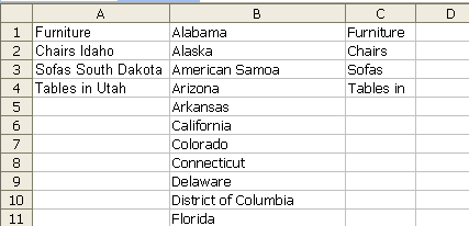
In A1:A3: Idaho, South Dakota, Utah
In B1: Furniture Chairs Idaho Sofas South Dakota Tables in Utah
In C1:=TRIM(SUBSTITUTE(B1,INDEX($A$1:$A$56,IF(ISNA(MATCH(FALSE,ISERR(FIND($A$1:$A$56,B1)),FALSE)),0,MATCH(FALSE,ISERR(FIND($A$1:$A$56,B1)),FALSE)),1),””))
Copy C1 to the right all the way to E1. That’s more or less what you did. Now…
Copy everything inside the TRIM function from D1. In E1, replace every instance of D1 with what you copied. While you’re in edit mode, you’ll see the outline around D1 disappear and you’ll know you got them all.
Then copy everything inside the TRIM function in C1. In E1, replace every instance of C1 with what you copied. There are a lot of them.
When the only edit-mode outlines you see are around A1:A4 and B1, you got them all.
Oh, yeah. I tried to do this without the copy/replace method. That is, by hand. But I gave up rather quickly.
You could also use IFERROR instead of ISNA and that would help a little. I’m not sure you get to 10 levels deep though.
Thank you so very much… Not only does your formula address my requested need, you also provided a very clear and understandable step-by-step instructions to achieving my goals.
As per you mentioning, it does not necessarily allow me to go beyond 10 levels of text removal/extraction per formula (which is perfectly fine), but does allow me to remove 3 keywords at a time as provided in the range/list. This greatly reduces (3x) the number of times I need to go across to each cell.
Lastly, I was able to successfully add one additional nested formula to the existing one, unfortunately, MS Excel does not allow you to go beyond the maximum characters per cell.
Thanks.
For your review and future use to anyone seeking this method, I’ve provided below:
=TRIM(SUBSTITUTE(SUBSTITUTE(SUBSTITUTE(SUBSTITUTE(B1,INDEX($A$1:$A$56,IF(ISNA(MATCH(FALSE,ISERR(FIND($A$1:$A$56,B1)),FALSE)),0,MATCH(FALSE,ISERR(FIND($A$1:$A$56,B1)),FALSE)),1),””),INDEX($A$1:$A$56,IF(ISNA(MATCH(FALSE,ISERR(FIND($A$1:$A$56,SUBSTITUTE(B1,INDEX($A$1:$A$56,IF(ISNA(MATCH(FALSE,ISERR(FIND($A$1:$A$56,B1)),FALSE)),0,MATCH(FALSE,ISERR(FIND($A$1:$A$56,B1)),FALSE)),1),””))),FALSE)),0,MATCH(FALSE,ISERR(FIND($A$1:$A$56,SUBSTITUTE(B1,INDEX($A$1:$A$56,IF(ISNA(MATCH(FALSE,ISERR(FIND($A$1:$A$56,B1)),FALSE)),0,MATCH(FALSE,ISERR(FIND($A$1:$A$56,B1)),FALSE)),1),””))),FALSE)),1),””),INDEX($A$1:$A$56,IF(ISNA(MATCH(FALSE,ISERR(FIND($A$1:$A$56,SUBSTITUTE(SUBSTITUTE(B1,INDEX($A$1:$A$56,IF(ISNA(MATCH(FALSE,ISERR(FIND($A$1:$A$56,B1)),FALSE)),0,MATCH(FALSE,ISERR(FIND($A$1:$A$56,B1)),FALSE)),1),””),INDEX($A$1:$A$56,IF(ISNA(MATCH(FALSE,ISERR(FIND($A$1:$A$56,SUBSTITUTE(B1,INDEX($A$1:$A$56,IF(ISNA(MATCH(FALSE,ISERR(FIND($A$1:$A$56,B1)),FALSE)),0,MATCH(FALSE,ISERR(FIND($A$1:$A$56,B1)),FALSE)),1),””))),FALSE)),0,MATCH(FALSE,ISERR(FIND($A$1:$A$56,SUBSTITUTE(B1,INDEX($A$1:$A$56,IF(ISNA(MATCH(FALSE,ISERR(FIND($A$1:$A$56,B1)),FALSE)),0,MATCH(FALSE,ISERR(FIND($A$1:$A$56,B1)),FALSE)),1),””))),FALSE)),1),””))),FALSE)),0,MATCH(FALSE,ISERR(FIND($A$1:$A$56,SUBSTITUTE(SUBSTITUTE(B1,INDEX($A$1:$A$56,IF(ISNA(MATCH(FALSE,ISERR(FIND($A$1:$A$56,B1)),FALSE)),0,MATCH(FALSE,ISERR(FIND($A$1:$A$56,B1)),FALSE)),1),””),INDEX($A$1:$A$56,IF(ISNA(MATCH(FALSE,ISERR(FIND($A$1:$A$56,SUBSTITUTE(B1,INDEX($A$1:$A$56,IF(ISNA(MATCH(FALSE,ISERR(FIND($A$1:$A$56,B1)),FALSE)),0,MATCH(FALSE,ISERR(FIND($A$1:$A$56,B1)),FALSE)),1),””))),FALSE)),0,MATCH(FALSE,ISERR(FIND($A$1:$A$56,SUBSTITUTE(B1,INDEX($A$1:$A$56,IF(ISNA(MATCH(FALSE,ISERR(FIND($A$1:$A$56,B1)),FALSE)),0,MATCH(FALSE,ISERR(FIND($A$1:$A$56,B1)),FALSE)),1),””))),FALSE)),1),””))),FALSE)),1),””),INDEX($A$1:$A$56,IF(ISNA(MATCH(FALSE,ISERR(FIND($A$1:$A$56,SUBSTITUTE(SUBSTITUTE(SUBSTITUTE(B1,INDEX($A$1:$A$56,IF(ISNA(MATCH(FALSE,ISERR(FIND($A$1:$A$56,B1)),FALSE)),0,MATCH(FALSE,ISERR(FIND($A$1:$A$56,B1)),FALSE)),1),””),INDEX($A$1:$A$56,IF(ISNA(MATCH(FALSE,ISERR(FIND($A$1:$A$56,SUBSTITUTE(B1,INDEX($A$1:$A$56,IF(ISNA(MATCH(FALSE,ISERR(FIND($A$1:$A$56,B1)),FALSE)),0,MATCH(FALSE,ISERR(FIND($A$1:$A$56,B1)),FALSE)),1),””))),FALSE)),0,MATCH(FALSE,ISERR(FIND($A$1:$A$56,SUBSTITUTE(B1,INDEX($A$1:$A$56,IF(ISNA(MATCH(FALSE,ISERR(FIND($A$1:$A$56,B1)),FALSE)),0,MATCH(FALSE,ISERR(FIND($A$1:$A$56,B1)),FALSE)),1),””))),FALSE)),1),””),INDEX($A$1:$A$56,IF(ISNA(MATCH(FALSE,ISERR(FIND($A$1:$A$56,SUBSTITUTE(SUBSTITUTE(B1,INDEX($A$1:$A$56,IF(ISNA(MATCH(FALSE,ISERR(FIND($A$1:$A$56,B1)),FALSE)),0,MATCH(FALSE,ISERR(FIND($A$1:$A$56,B1)),FALSE)),1),””),INDEX($A$1:$A$56,IF(ISNA(MATCH(FALSE,ISERR(FIND($A$1:$A$56,SUBSTITUTE(B1,INDEX($A$1:$A$56,IF(ISNA(MATCH(FALSE,ISERR(FIND($A$1:$A$56,B1)),FALSE)),0,MATCH(FALSE,ISERR(FIND($A$1:$A$56,B1)),FALSE)),1),””))),FALSE)),0,MATCH(FALSE,ISERR(FIND($A$1:$A$56,SUBSTITUTE(B1,INDEX($A$1:$A$56,IF(ISNA(MATCH(FALSE,ISERR(FIND($A$1:$A$56,B1)),FALSE)),0,MATCH(FALSE,ISERR(FIND($A$1:$A$56,B1)),FALSE)),1),””))),FALSE)),1),””))),FALSE)),0,MATCH(FALSE,ISERR(FIND($A$1:$A$56,SUBSTITUTE(SUBSTITUTE(B1,INDEX($A$1:$A$56,IF(ISNA(MATCH(FALSE,ISERR(FIND($A$1:$A$56,B1)),FALSE)),0,MATCH(FALSE,ISERR(FIND($A$1:$A$56,B1)),FALSE)),1),””),INDEX($A$1:$A$56,IF(ISNA(MATCH(FALSE,ISERR(FIND($A$1:$A$56,SUBSTITUTE(B1,INDEX($A$1:$A$56,IF(ISNA(MATCH(FALSE,ISERR(FIND($A$1:$A$56,B1)),FALSE)),0,MATCH(FALSE,ISERR(FIND($A$1:$A$56,B1)),FALSE)),1),””))),FALSE)),0,MATCH(FALSE,ISERR(FIND($A$1:$A$56,SUBSTITUTE(B1,INDEX($A$1:$A$56,IF(ISNA(MATCH(FALSE,ISERR(FIND($A$1:$A$56,B1)),FALSE)),0,MATCH(FALSE,ISERR(FIND($A$1:$A$56,B1)),FALSE)),1),””))),FALSE)),1),””))),FALSE)),1),””))),FALSE)),0,MATCH(FALSE,ISERR(FIND($A$1:$A$56,SUBSTITUTE(SUBSTITUTE(SUBSTITUTE(B1,INDEX($A$1:$A$56,IF(ISNA(MATCH(FALSE,ISERR(FIND($A$1:$A$56,B1)),FALSE)),0,MATCH(FALSE,ISERR(FIND($A$1:$A$56,B1)),FALSE)),1),””),INDEX($A$1:$A$56,IF(ISNA(MATCH(FALSE,ISERR(FIND($A$1:$A$56,SUBSTITUTE(B1,INDEX($A$1:$A$56,IF(ISNA(MATCH(FALSE,ISERR(FIND($A$1:$A$56,B1)),FALSE)),0,MATCH(FALSE,ISERR(FIND($A$1:$A$56,B1)),FALSE)),1),””))),FALSE)),0,MATCH(FALSE,ISERR(FIND($A$1:$A$56,SUBSTITUTE(B1,INDEX($A$1:$A$56,IF(ISNA(MATCH(FALSE,ISERR(FIND($A$1:$A$56,B1)),FALSE)),0,MATCH(FALSE,ISERR(FIND($A$1:$A$56,B1)),FALSE)),1),””))),FALSE)),1),””),INDEX($A$1:$A$56,IF(ISNA(MATCH(FALSE,ISERR(FIND($A$1:$A$56,SUBSTITUTE(SUBSTITUTE(B1,INDEX($A$1:$A$56,IF(ISNA(MATCH(FALSE,ISERR(FIND($A$1:$A$56,B1)),FALSE)),0,MATCH(FALSE,ISERR(FIND($A$1:$A$56,B1)),FALSE)),1),””),INDEX($A$1:$A$56,IF(ISNA(MATCH(FALSE,ISERR(FIND($A$1:$A$56,SUBSTITUTE(B1,INDEX($A$1:$A$56,IF(ISNA(MATCH(FALSE,ISERR(FIND($A$1:$A$56,B1)),FALSE)),0,MATCH(FALSE,ISERR(FIND($A$1:$A$56,B1)),FALSE)),1),””))),FALSE)),0,MATCH(FALSE,ISERR(FIND($A$1:$A$56,SUBSTITUTE(B1,INDEX($A$1:$A$56,IF(ISNA(MATCH(FALSE,ISERR(FIND($A$1:$A$56,B1)),FALSE)),0,MATCH(FALSE,ISERR(FIND($A$1:$A$56,B1)),FALSE)),1),””))),FALSE)),1),””))),FALSE)),0,MATCH(FALSE,ISERR(FIND($A$1:$A$56,SUBSTITUTE(SUBSTITUTE(B1,INDEX($A$1:$A$56,IF(ISNA(MATCH(FALSE,ISERR(FIND($A$1:$A$56,B1)),FALSE)),0,MATCH(FALSE,ISERR(FIND($A$1:$A$56,B1)),FALSE)),1),””),INDEX($A$1:$A$56,IF(ISNA(MATCH(FALSE,ISERR(FIND($A$1:$A$56,SUBSTITUTE(B1,INDEX($A$1:$A$56,IF(ISNA(MATCH(FALSE,ISERR(FIND($A$1:$A$56,B1)),FALSE)),0,MATCH(FALSE,ISERR(FIND($A$1:$A$56,B1)),FALSE)),1),””))),FALSE)),0,MATCH(FALSE,ISERR(FIND($A$1:$A$56,SUBSTITUTE(B1,INDEX($A$1:$A$56,IF(ISNA(MATCH(FALSE,ISERR(FIND($A$1:$A$56,B1)),FALSE)),0,MATCH(FALSE,ISERR(FIND($A$1:$A$56,B1)),FALSE)),1),””))),FALSE)),1),””))),FALSE)),1),””))),FALSE)),1),””))
Excel only allows 64 levels of nesting. Is there a way to make this work for more substitutions, like 400, without using vba code? Normally, in each cell there will not be more than 5 strings to substitute but those are 5 from the possible 400 ones.
Changing “01A039 600100 100101” into “01,A,039,60,02,00,10,01”?
I can use MID but for the sake of learning new ways can it be done with a formula (no VBA) that gets as one of the arguments an array with the positions for inserting the commas?
01, not 02. Sorry. Could you please modify the original comment, so that it goes in one place?
Sorry again, please don’t allow my comments.😓
If you find a solution, just make an article.
For example:
=MID(A1,{1,3,4,8,10,12,15,17,19},{2,1,3,2,2,2,2,2,2})&comma
generates a beautiful array, but how to concatenate it?
=TEXTJOIN("",TRUE,MID(A1,{1,3,4,8,10,12,15,17,19},{2,1,3,2,2,2,2,2,2})&",")How about using a recursive array formula to recursively substitute? In C1, try this formula:
=IF((((C1=0)+(C1=C$1))*1),TRIM(A1),SUBSTITUTE(TRIM(C1),INDEX($B$1:$B$50,MAX(IF(ISNUMBER(FIND($B$1:$B$50,C1)),ROW(INDIRECT(“$1:$”&ROW($B$50))),0))),””))
This needs to be array-entered (using Ctrl+Shift+Enter)
Iterative calculations need to be enabled in Excel Options > Formulas > Calculation Options > Enable Iterative calculation