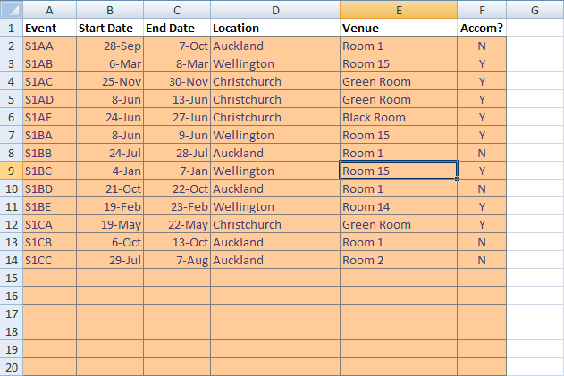
Nothing wrong with this sheet, right?

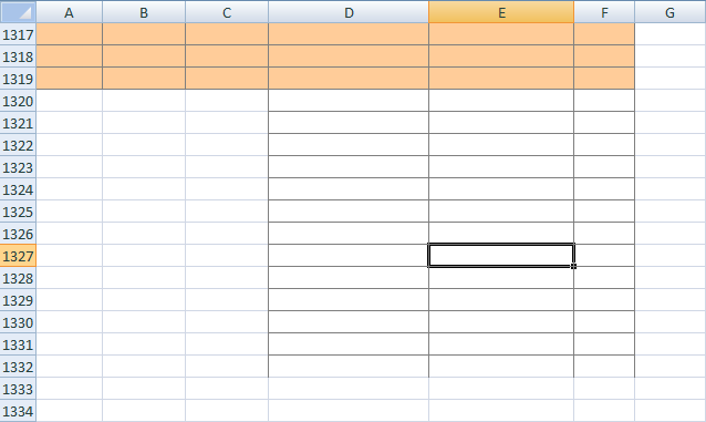
Until you get to the end…

The teeny-tiny vertical scrollbar handle is usually a give away. Hundreds of rows tacked onto the end of the list to give the illusion that the whole column has been formatted.
The trouble with formatting columns as per the above image is that it causes the “last used row” to be hundreds of rows further down than necessary. Click print and you waste a forest. It could also cause your workbook file size to bloat! In any case the vertical scrollbar’s usefulness takes a serious blow.
The answer is to format not individual cells, but the whole column.
– Select the worksheet column (or columns). The short-cut key is Ctrl+Space. In the above example, we’d highlight columns A to F.
– Right-click the selection, and choose Format Cells…
– Apply formatting the way you want.
If we did this exercise on the above example, you would notice that the column headers would also be formatted the same as the content, which is often not what we want. The trick is to format them last.
So the general order of formatting goes:
– Format the whole sheet
– Format the whole column
– Format just the column header (label)
Hopefully this diagram explains it.

This method allows your worksheet to grow while maintaining consistent formats for new rows.
Rob,
I thought the last cell was dictated by the bottom-right-most cell with formatting. I often need to take others’ workbooks and delete the unused rows and columns to get the file to a reasonable size. Your post indicates that you can format an entire sheet without bloating the file size. Is the trigger for the last cell only number formatting?
A bit confused
Brett
Hi,
Look like a great tric but I can’t seem to get it to work in Excel 2003. Does it also work in that version?
Thx
Tom
No, it may also be a cell you entered data into and subsequently cleared. Excel will keep that cell as the last used.
You have to remember how Excel remembers formatting.
Whole sheet formatting requires one set of settings for the whole sheet.
Whole row or column formatting requires one set of settings for the whole row or column.
Arbitrary range formatting requires one set of settings for each cell in the range.
It is this last category that helps to define the last cell, and which consumes the majority of formatting resources.
Brett: It is true that you can format the entire sheet without bloating file size.
As a simple experiment, using Excel 2003, I coloured the entire sheet (A1:IV65536) in one workbook, and saved.
In a another new workbook, I coloured cells A1:IU65535 (one row and one column short of the entire sheet), and saved.
14 kilobytes for the whole sheet
34 megabytes for the partial sheet
I have another solution: format ONLY ROWS that have data in it.
1. Select only the columns that you want it to apply to
(For example,
=$A:$Z
)
2. In Office 2007, on the “Home” tab, select “Conditional FormattingNew Rule…”
3. Under “Select a Rule Type:” pick “Use a formula to determine which cells to format”
4. Apply the following formula:
=NOT(ISBLANK($A1))
(In my case I used column A, but use whatever column you are sure will have data in each row of records, don’t use a column that might have blank cells in it. Realize that the row won’t format until there is a value in the column that you choose).
5. Select the formatting
(E.g. font = Arial 10, border = outline, fill = grey)
6. (Optional) I like to hide the grid lines, giving a contrast between the cells with border outlines and a white, blank sheet – it adds a slick look to the file! Simply uncheck “Show Gridlines” under Excel OptionsAdvancedDisplay Options for this worksheet
VARIATION FOR SHEET WITH HEADER ROW
If you are using the first row as a header row, and want the formatting to apply only to rows below the first row, change the area you select and tweak the formula.
If you use the mouse to select the area, select all the columns, then Ctrl-click the first row to exclude it from the selection. If you want to type it in, it would look something like this:
=$A:$Z,$1:$1
tweak the formula to accommodate the offset of the header row:
=NOT(ISBLANK($A2))
Now you can apply whatever formatting you want to the first row, add filters and freeze the top row if desired.
Voila! Hope you’ve found this helpful :-)
hi,
I have one inventry related work sheet.
in that sheet my product code is in sheet1 & my query sheet is sheet 6
i need sheet 6 if B3=blank than a3=”NR” if B3= ‘sheet1!”product code” than a3=”D” and if b3 notequal to ‘sheet1!”product code” than a3=”P”
how can i do?
i also try this formula =IF(ISBLANK(B3),”NR”,IF(B3=’CHECK DELTA’!$A$3:$A$50000,”D”,”P”)) but is not working.
ashish:
=IF(ISBLANK(B3), “NR”, IF(NOT(ISNA(MATCH(B3, ‘CHECK DELTA’!$A$3:$A$50000, 0))), “D”, “P”))
Rob, i think what Angela said was right, have you try it out?
Hi,
Thanks Rob, Stuart & Angela.
Angela: very useful and innovative. Thanks!