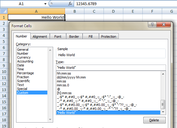
It is possible to get a cell to display one thing, but store another.
Create a Custom Format by right-clicking the cell, select Format Cells…, then from the Number tab select Custom.
In the Type box use whatever text you want displayed, but be sure to enclose it in “double-quotes”.

I admit, this is a pretty dirty trick, but it may have legit uses.
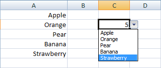
Data Validation cell dropdowns also use this format. This makes it possible to select a text value from a list, but it will store the number instead!

There’s probably a limit to the number of custom formats. I’m not sure what that limit is, but I reckon it’s big, because in many of the spreadsheets I’ve worked on there are way, way too many.
This trick has some very interesting uses I’ve used before. Unfortunately the limit of custom formats is 256 and has not been increased in 2007 like so many other limits. Maybe in 2010? haven’t checked yet.
Interesting. how does that validation you show has to be set up?
A1 is 1, A2 is 2, A3 is 3, A4 is 4, A5 is 5
Custom Format for A1 is “Apple”, A2 is “Orange”, A3 is “Pear”, A4 is “Banana”, A5 is “Strawberry”
A simple list dropdown using Data Validation, using A1:A5 as the source. Excel does the rest.
It makes sense. It’s like how you can have a dropdown list of percentages, you select 50%, but it stores 0.5 instead.
awesome trick!
Neat. Something to use when you have tables in Excel that in fact need to go into a relational database with indexes for some fields instead of actual lookup values.
Another interesting behaviour
a1 : custom format is [>10]”big”;[>-10]”OK”;”small”
we get
A1 = 15 see : big
A1 = 5 OK
A1 = -5 -OK ???
A1 = -15 -small ???
but when custom format is [>10]”big”;[<-10]”small”;”OK”
we get
A1 = 15 see : big
A1 = 5 OK
A1 = -5 -OK ???
A1 = -15 small
Is it property or bug?
@Petrak
It’s math!
In your first scenario, only 15 is > 10, thus “big”
Both 5 and -5 are > -10, so “ok”
-15 does not meet any criteria, thus “small”
Similarly, in your second scenario,
only 15 is > 10, thus “big”
only -15 is < -10, thus “small”
5 and -5 do not meet either criteria, thus “ok”.
@JKP – you jest surely! Why would you just not store the list and do a MATCH to get its index if you want an index value?
This strikes me as a mildly amusing trick that has no real practical use, nothing that cannot be achieved more easily and clearly in other ways.
The only time I’ve ever used this was in a Calendar to disguise the basis date. Beside that, I think it’s dirty, but worth of knowing.
So says the man who disparaged array formulae
There was a grin at the end of that last comment, don’t know where it went.
Bob: I’m reknown for my jokes :-))
I haven’t used it to hide values but to format formula results, ie:
“Answer is” #### “dollars”
I use this when I want the user to visualize a boolean and the model I’m building is checking only whether the custom-formatted cell is blank. I use a capital X in quotes as the format. Occasionally I use it for April Fool’s day fun.
Brett
@ Luke M, Petrak has no problem with the maths. He has a question with what is displayed when the different formats are applied.
a1 : custom format is [>10]”big”;[>-10]”OK”;”small”
we get
A1 = 15 see : big
A1 = 5 OK
A1 = -5 -OK ??? this displays “-OK”
A1 = -15 -small ??? this displays “-small”
but when custom format is [>10]”big”;[<-10]”small”;”OK”
we get
A1 = 15 see : big
A1 = 5 OK
A1 = -5 -OK ??? this displays “-OK”
A1 = -15 small
Is it property or bug?