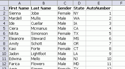
Let’s say you have some data like, oh I don’t know, First Name, Last Name, Gender, State, and some number.

You could add up the numbers for all the males in Texas with an array formula.
If you didn’t know that, go read Anatomy of an Array Formula. One of my workshop attendees had this situation except that she wasn’t hardcoding the values ‘Male’ and ‘Tx’. Instead she was getting those values from a cell that had a data validation drop down list. Also in that list was the word ‘All’, which of course meant to include everything from that column.
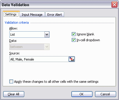
For this example, I set up data validation to include All, Male, and Female.

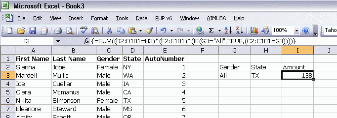
And I changed my array formula to this

The IF statement says: If G3 is All, then return TRUE no matter what’s in that column. If it’s not All, return TRUE for only those rows that match G3.
Normally in array formula, we multiply one array times another. The first element of array 1 is multiplied by the first element of array 2. The second element of array 1 is multiplied by the second element of array 2. And so on for every element. When we multiply an array by a scalar value (like TRUE in this example), then each element of the array is multiplied by that scalar value. That allows us to return TRUE for every Gender, thereby ignoring that column.
As ever, you can do a non-array form
=SUMPRODUCT(((G3=”All”)+(C2:C101=G3))*(D2:D101=H3),E2:E101)
and two whole characters shorter (:-))
Actually yours can be used in the same way, sans IF,
=SUM(((G3=”All”)+(C2:C101=G3))*(D2:D101=H3)*(E2:E101))
whiche is 5 characters shorter yet, but still a nasty array formula.
Another fancy trick. Excel is talented, versatile, powerful, is “younger than I am yet it is more popular, worth more money, has more homes, is touched by more women, and is far better at math.” (Mike Rouse on Excel’s 21st birthday, 5 Sept 2006).
The beauty of this formula is that it makes quantitative sense of a data set by letting Boolean and numeric values work indiscriminately together.
At least one product sign is essential: {=SUM((D2:D101=”NY”)*1)} makes sense whereas {=SUM(D2:D101=I12)} doesn’t, same for =SUMPRODUCT(…), which makes us think these functions were written for multiple condition scenarios.
The plus condition is perfect. I hate IFs in my array formulas.
So do I, but sometimes they are a necessary evil. Sometimes you just have to outsort the data otherwise it errors. Then you have to use IF, there is no other way I can think of.
Hi Dick,
I have some trouble with array formula and as usual I went on your blog looking for some hint: amazingly enough you are talking about Array Formulas…
Does anybody know about any limitation in using array formulas? As far I can see Excel seems to behave inconsistently (i.e. I’m wrong, but I can’t get why): if I type the following (fictious) array formula
=SUM(ROW(1:5))
I get 15
If I type
=COUNT(ROW(1:5))
I get 5 (wow!)
If I type
=VLOOKUP(2,ROW(1:5),1,0)
I get 2 (Great!)
If I type
=rank(1,ROW(1:5),0)
I get an error (!!!???)
The same behaviour occurs when I try to use sumifs countifs and other formulas.
How can you explain this behaviour?
AleV, Excel Help has always been wrong about the RANK function. It’s 2nd argument MUST be a range reference; it can’t be an array.
Thanks fzz.
I’m just a little bit confused as I used to think that since Named Ranges are essentially (in general array) formulas (as Jhon Walkenbach notes in his books, they are entered by using a “=” sign in the Name Manager, so they ARE actually formulas), then they should not be different from other array formulas you can write (and enter in the Name Manager). Apparently my conclusion is wrong: the RANK function (like sumifs and others) can manage Named Ranges but not arrays.
Thanks again,
AleV
AleV – it’s the SYNTAX of the RANK function that REQUIRES that its 2nd argument be a range. Nothing to do with formula syntax.
To the general point, if recalc speed were the top priority, wouldn’t
=SUM(IF(G3=”All”,D2:D101=H3,(D2:D101=H3)*(C2:C101=G3))*E2:E101)
be the optimal approach? I’d use SUMPRODUCT myself, something more general like
=SUMPRODUCT(((G3=”All”)+(C2:C101=G3)>0)*(D2:D101=H3),E2:E101)
In the current inclusive, nonjudgmental, bioengineered age, one may need to allow for All as a possible entry for Sex.
Instead of using unnamed ranges like D2:D101 it’s better to use named dynamic ranges. You can substitute D2:D101 with cState where cState is named range =OFFSET(Book3!$D$1,1,0,COUNTA(Book3!$A:$A)-1,1). That makes your formulas easier to read as they are in pure English and you don’t have to worry what happens if your data range extends – especially useful when you get your data range from an external source.