I need help. I have this:
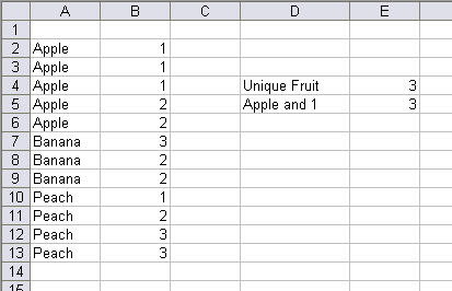
I can tell my how many unique fruits are in column A with this array formula
E4: =SUM(1/COUNTIF(A2:A13,A2:A13))
And I can tell how many rows have both Apple in column A and 1 in column B with this array formula
E5: =SUM((A2:A13=”Apple”)*(B2:B13=1))
But I can’t seem to figure out the formula to tell me the count of unique fruits that have a 1 in column B. The answer is two, apple and peach. What’s the formula that gets me there?
=SUMPRODUCT((A2:A13=”Apple”)*(B2:B13=1)+(A2:A13=”Peach”)*(B2:B13=1))
try (Ctrl+Shift+Enter):
=SUM(1*(MATCH(IF(B2:B13=1,A2:A13,””),IF(B2:B13=1,A2:A13,””),0)=ROW(INDIRECT(“1:”&ROWS(A2:A13)))))-1
Stolen from Chip’s site:
=SUM(IF(FREQUENCY(IF(LEN(IF(B2:B13=1,A2:A13,””))>0,MATCH(IF(B2:B13=1,A2:A13,””),IF(B2:B13=1,A2:A13,””),0),””),
IF(LEN(IF(B2:B13=1,A2:A13,””))>0,MATCH(IF(B2:B13=1,A2:A13,””),IF(B2:B13=1,A2:A13,””),0),””))>0,1))
Jamie.
If you enter in c2 the formula =A2&B2 and drag it to c13
then the answer can be :
{=SUM(1*(RIGHT(C2:C13)=”1?)*(1/COUNTIF(C2:C13,C2:C13)))}
You really should post such queries on the public NGs Dick, you would have been swamped with answers in minutes.
FROM (
SELECT F1 AS fruit_name
FROM [EXCEL 8.0;HDR=NO;IMEX=1;DATABASE=C:TempoDB.xls;].[Sheet4$A2:B13]
WHERE F2 = 1
GROUP BY F1
) AS DT1;
Hi Dick –
If you sort on B2:B13 ascending or your data is entered such that Apple 1 will be above Apple 2 and Peach 1 above Peach 2 etc, then
=SUMPRODUCT((B2:B13=1),(A2:A13A1:A12))
works.
Non-array alternate for E5: =SUMPRODUCT((A2:A13=”Apple”),(B2:B13=1))
…Michael
ps. A learning experience: When I copied the original E5 formula and pasted it into my spreadsheet it didn’t work. Took me a while to find that the problem was that from the web, it comes over with curly quotes.
Why even post in newsgroups? Why not just search them? This has been asked AND ANSWERED many times. But I suppose bloggers can choose to reinvent wheels whenever they want. So WTH,
=COUNT(1/FREQUENCY(MATCH(Fruits,Fruits,0)*(Numbers=1),
ROW(Fruits)-MIN(ROW(Fruits))))-1
More generally,
=COUNT(1/FREQUENCY(MATCH(IDs,IDs,0)*CriteriaArray,
ROW(IDs)-MIN(ROW(IDs))))-1
BTW, I liked the SQL answer, especially the Jet-centric nature of it, requiring a nested query rather than the more direct
SELECT Count(Distinct Fruit)
FROM TableHoweverSpecified
WHERE Number=1;
that’s possible using real SQL RDBMSs.
Hey Jamie I thought you didn’t trust the Excel SQL. (External Data – Mixed Data Types 2004 3rd June) but I admire the originality. But surely it should be.
SELECT F1
FROM Table1
GROUP BY F1, F2=1
HAVING (F2=1)=True
Without restrictions, this should be the easiest:
=SUM(1/COUNTIF(C2:C13;C2:C13))-1
Column C: =IF(B2=1;A2)
//Ola
This is a harder calculation to make foolproof than it appears.
fzz’ COUNT and FREQUENCY formula is nice because it does not require array entry. However, it underpredicts by 1 if every entry in Fruits is unique and every value in Numbers is 1. And it will return -1 if there are one or more blanks in Fruits.
Ioannis Varlamis’ formula underpredicts by 1 when every entry in Fruits is unique and every value in Numbers is 1. Otherwise, it works.
The formula on Chip’s site (as cited by Jamie Collins) handles the above cases, but underpredicts by 1 when one of the Fruits is blank but its Numbers is still 1. This somewhat shorter array formula behaves similarly. It assumes row 14 is either blank, has a duplicate Fruits or Numbers does not equal 1:
=SUM((N(MATCH(IF(B2:B14=1, A2:A14,””),IF(B2:B14=1, A2:A14,””),0)=ROW(A2:A14)-ROW(A$2)+1)))-1
Brad
Jan: “Hey Jamie I thought you didn’t trust the Excel SQL”
Very observant, but my true feelings on this (i.e. put the data in a SQL DBMS) is probably OT for an Excel blog .
Note I used
merely to get a distinct set e.g. could also have done this:
FROM Table1
WHERE F2 = 1;
A
clause is normally reserved for predicates involving set functions; your
(no need for
) can and IMO should go in the
clause e.g. consider this contrived example:
FROM Table1
WHERE F2 = 1
GROUP BY F1, F2
HAVING COUNT(*) > 1;
The COUNT(*) cannot be evaluated in the
clause, hence the need for a
clause.
I recently read a paper by Hugh Darwen, in which he ponders whether
would be in the SQL language at all if early SQL DBMSs had supported derived tables e.g. contrast this to the above:
FROM (
SELECT F1 AS fruit_name, F2 AS foo, COUNT(*) AS bar_tally
FROM Table1
GROUP BY F1, F2
) AS DT1
WHERE DT1.bar_tally > 1;
Jamie.
Please ignore my previous post I must have been drunk.
When I use it properly “Having” is much more elegant than the sub select.
Jan, That’s one of my least favourite Per Gessle songs (“It must have been lunch but I’m sober now…”)
Sure,
is elegant and a ‘nice to have’ feature but non-essential and one that confused the heck out of me as a newbie.
Jamie.
Brilliant, just what I was looking for and needed this very day, thanks to all, saved me loads of time.
Byundt, thanks for remark.
Perhaps, better:
=SUM(1*((MATCH(A2:A13,A2:A13,0)=ROW(INDIRECT(“1:”&ROWS(A2:A13))))+(B2:B13=1)=2))
(Ctrl+Shift+Enter)
Ioannis
Give a ty to this.
=SUMPRODUCT((B2:B13=1),(MATCH(A2:A13&”#”&B2:B13,A2:A13&”#”&B2:B13,0)=ROW(A2:A13)-ROW(A2)+1))
Saludos
Just shortend, Elias formula:
=SUM((B2:B13=1)*(MATCH(A2:A13;A2:A13;0)=ROW(A2:A13)-ROW(A2)+1))
As a bonus, it makes it easy to add a 3rd, 4th, … column with restrictions.
//Ola Sandström
Hola Ola,
Your formula isn’t working; to use this kind of formula you should concatenate the two columns to find a unique entry.
Saludos
Elias, it must have been too early in the morning. Thanks for spotting that.
//Ola
It could be interesting to know that Google now supports Array formulas.
http://google-d-s.blogspot.com/2007/07/array-formulas-without-ctrl-shift-enter.html
Example:
=ARRAYFORMULA(SUMPRODUCT((B3:B14=1)*(MATCH(A3:A14&”#”&B3:B14;A3:A14&”#”&B3:B14;0)=ROW(A3:A14)-ROW(A3)+1)))
=ARRAYFORMULA(SUM((N(MATCH(IF(B3:B14=1,0;A3:A14;””);IF(B3:B14=1,0;A3:A14;””);0,0)=ROW(A3:A14)-ROW(A$3)+1,0)))-1,0)
Both works when imported: http://spreadsheets.google.com/pub?key=pAxhcqJ1DpABcRxoPqKNFYw
However Zoho seams to have problems
http://web.omnidrive.com/APIServer/public/8qr1RsuHYalOM7wsHSHS4J8w/UniqueFruits2.xls
//Ola
Dick I know it isn’t Excel but I think we need another look at Google Spreadsheets vs Excel article (things have come along in the last year since you last looked at it and to be fair the last article was a bit sparse). We all know this is going to have a long term effect on the Microsoft strangle hold and I would hate to be caught out.
The other day I bought a computer and I dreaded loading all my stuff back on, but it turns out it was a breaze. Nearly everything I needed was already on the web, except MS Office. Then I remembered that other than for work, I didn’t even need that ! How long till all my stuff is on-line at Google?
I must say that the ARRAYFORMULA is a smart move by Google (maybe inspired by TED.com).
It’s the sort of thing the computer press would write about – it’s a good story.
If your thinking of it, I have a fresh zip-file with documents from Zoho, OpenOffice and Google that might help:
http://web.omnidrive.com/APIServer/public/8qr1RsuHYalOM7wsHSHS4J8w/Spreadsheet_Functions.zip
//Ola
The best formula is the one you are able to use. Ugliness can be interesting insofar it is functional, but in general, simple is beautiful and desirable in the face of a problem.
From the formulae that solve Dick’s problem as it is, and whithout blanks, the shortest one is 51 characters long, the longest (from Chip pearson’s website) has 207 characters. The one formula I will remember is avner’s; the fact that he concatenates the two colums, to me, just makes his solution more elegant:
=SUM(1*(RIGHT(c2:c13)=”1?)*1/COUNTIF(c2:c13,c2:c13))
The non-array form is longer (58 chars) but just as simple:
=SUMPRODUCT((RIGHT(c2:c13)=”1?)*1,1/COUNTIF(c2:c13,c2:c13))
FTHOI, more robust.
=COUNT(1/FREQUENCY(MATCH(Fruits&””,Fruits&””,0)
*(Fruits””)*(Numbers=1),ROW(Fruits)-MIN(ROW(Fruits))))
-(SUMPRODUCT(1/COUNTIF(Fruits,Fruits&””),
(Fruits””)*(Numbers=1))
@#$% edit box!
FTHOI, more robust.
=COUNT(1/FREQUENCY(MATCH(Fruits&””,Fruits&””,0)
*(Fruits<>””)*(Numbers=1),ROW(Fruits)-MIN(ROW(Fruits))))
-(SUMPRODUCT(1/COUNTIF(Fruits,Fruits&””),
(Fruits<>””)*(Numbers=1))<ROWS(Fruits))
Ola: does ThinkFree’s spreadsheet handle array formulas?
fzz: Not as good as Google. I took the spreadsheet that I used before and imported it to ThinkFree-Calc. Half of the array formulas worked. Ctrl+Shift+Enter works, but I had to use that to make SUMPRODUCT work so somehow, Googles solution feels more robust. What speaks for ThinkFree is that it has the best ‘Excel feeling’ to it and the graphics that was imported in the spreadsheet came along just perfect.
I made a quick update of the formula comparison sheet (ThinkFree is now included): http://web.omnidrive.com/APIServer/public/8qr1RsuHYalOM7wsHSHS4J8w/Spreadsheet_Functions2.zip
This made me think, maybe there should be an acid-test spreadsheet here. It could be a good challenge for all developers. My second thought was, what happens when everyone come up to standard? Will we have a group of developers who will want to go further? Could we get that long sought integration of the Rocks and the Water (Juice Analytics)?
//Ola
Refined Jamie’s formula; no additional columns and works without reference to rows.
=SUM(IF(FREQUENCY(IF(B2:B13=1,MATCH(A2:A13,A2:A13,0),””),IF(B2:B13=1,MATCH(A2:A13,A2:A13,0),””))>0,1))
(Ctrl+Shift+Enter)
EditGrid is also included in the file. When if comes to number of formulas, no one beats EditGrid (500+).
If you like to try editgrid.com I made an open account – free for us (everyone). Lgn: ExcelUser Paswrd: ExcelUser (misspelled to avoid searchers). There is one file for now, UniqueFruits: http://www.editgrid.com/user/exceluser/UniqueFruits2 but you can test and upload any file, as long as it’s smaller than 2Mb.
//Ola
Ola,
I have been meaning to get around to a thorough side by side comparison for some time now. Thank you so much for doing this.
I will check in with our developers at ThinkFree to see about the Array formula problem you mentioned.
Are you planning on doing a similar comparison with charts and graphs or determining compatibility with Excel?
We definitely agree with you – EditGrid is a very cool spreadsheet application. ThinkFree Calc comes in two modes – Quick Edit (AJAX) and Power Edit (Java). We partnered with TnC (the makers of EditGrid) to have EditGrid replace our current version of Quick Edit Calc. Hopefully the integration will be done in the next month or so.
Thanks,
Jonathan
I’ve slightly refined Anthony’s refined version of Jamie’s formula :-)
=SUM(SIGN(FREQUENCY(IF(B2:B13=1,MATCH(A2:A13,A2:A13,0),””),IF(B2:B13=1,MATCH(A2:A13,A2:A13,0),””))))
(Ctrl+Shift+Enter)
I’m using it to count multiple columns on a large sheet, so processing speed/efficiency is an issue, and the SIGN(…) function is slightly more efficient than the IF(…,>0,1) function.
Jonathan,
Thanks for the appreciation. EditGrid and Thinkfree sounds like an interesting cooperation. I look forward to try the end result.
The “function comparison file” is now updated. It will never be 100% correct but it’s probably the best function comparison to date. The biggest problem was to handle the differences between the Manual and the User Interface (fx button). All suppliers have some updating to do.
Have I though about to do Charts and Graphs comparison? No, I could consider a small acid test for spreadsheet functions but not for charts and graphs. Someone else might feel inclined though?
I though I mention it also, ThinkFree often freezes my computer (had to reboot 3 times). So any improvement there would be appreciated.
zb,
I have taken the liberty to put your solution in an EditGrid test file (link below).
Dick,
I am sorry if you disapprove of this the conversation since it’s not related to your original post.
//Ola
Function comparison file: http://web.omnidrive.com/APIServer/public/8qr1RsuHYalOM7wsHSHS4J8w/Spreadsheet_Functions2.zip
Test file: http://www.editgrid.com/user/exceluser/UniqueFruits2
To edit the test file, see login/psw in the previous post
*IF* online spreadsheets made it relatively simple to process results of web queries via FORMULAS, provided some form controls for use inside worksheets, and provided hidden worksheets and protection so that only a spreadsheet’s creator ID could unprotect it, then I could see online spreadsheets as a fairly complete replacement for spreadsheet models that don’t need VBA/macros.
Naively, I’d assume it wouldn’t be too difficult for the online spreadsheets to provide these security features (hiding rows, columns, sheets and creator-only protect/unprotect). Actually, that alone would make it superior to Excel in terms of IP protection.
As for the latter, maybe a function named wget (after the Unix-originated utility of that same name) that would return whatever it’s url argument returned. In the short term, it’d be sufficient just to be able to enter the result as an array formula that could be accessed by other, parsing formulas.
Just thinking out loud.
Hello All –
Is it possible to determine the number of unique items in a filtered list? I wrote a UDF that returns TRUE() if the row is visible, but I can’t figure out the array to multiply it by, and I didn’t get anywhere using SUBTOTAL().
For instance, in Dick’s above example, if we filter on “Apple” I would like to know that of the three 1’s and two 2’s in Column B, there are just 2 unique values in Column B.
Thanks,
Michael
Michael,
Will you please share an example of the UDF you wrote that returns TRUE() if the row is visible?
Thanks, Dorothy
Hi Dorothy –
Couldn’t be much simpler. Glad to share.
Application.Volatile
IsVisible = Not Cell.EntireRow.Hidden
End Function
…Michael
if this is the source file;
apple 1
apple 2
apple 3
banana 2
banana 1
orange 1
orange 3
than using formula in excel,i want the result;
apple 1 2 3
banana 1 2
orange 1 3
someone help please…
Use:
=SUM((MATCH(A1:A12,A1:A12,0)=ROW(A1:A12))*(B1:B12=1))
if in A1:A12. You have to adjust the ROW matrix back to 1 for other ranges.
Hi All,
Taking the same example, I have to calculate number of rows where Column A has Apple and Column B has value 1. I am new to VBA scripts in Excel and I have dumped the following formula in cell B5 in the excel sheet:
=SUM((A2:A13=”Apple”)*(B2:B13=1))
The above formula is not working; the calculation/output of this formula is “0? and not “3? as shown in the Figure.
Simple steps to get the value “3? by using the above formula will help me a lot!!!!
Hope to see an early response!
Cheers Mam.
Mam,
You need to array-enter formulas like that:
1) Select the cell with the formula
2) Click in the formula bar
3) Hold the Control and Shift keys down
4) Hit the Enter key, then release it
5) Release the other two keys (Control and Shift)
Excel should respond by adding curly braces surrounding your formula. You don’t type theseExcel must add them for you.
{=SUM((A2:A13=”Apple”)*(B2:B13=1))}
If you do not array-enter the formula, then the result will be a test just of cells A2 and B2. That’s why you should have gotten 1 instead of 3 (when testing Dick’s sample data).
Incidently, the same syntax can be used with the SUMPRODUCT functionand you don’t need to array-enter the formula:
=SUMPRODUCT((A2:A13=”Apple”)*(B2:B13=1))
Brad
{=SUM(IFERROR((B2:B13=1)/COUNTIFS($B$2:$B$13,1,$A$2:$A$13,A2:A13),0))}
Hi David Hager,
A big fan of yours articles ! Thanks a lot !
Do you maintain any website ? Would love to visit.
Warm Regards
Kanwaljit
Kanwaljit says:
Do you maintain any website ? Would love to visit.
Not at this time. I will have some free time later this year, and if I come up with anything new and interesting, I will post it in this blog.