There has to be a better way than this, but I can’t think of it. I have a string with a capital letter somewhere in it and I need to determine the position of that letter. The goal is to strip out all the letters before it. The test subject is the string mdtTxnDate. The array formula that seems to work is:
It assumes that the capital letter won’t be more than 255 characters in, which is true in my case. This is an array formula, so it needs to be entered with Control+Shift+Enter, not just enter. Here’s the break down:
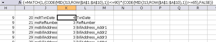
returns an array of ASCII characters that make up the string. Although it returns a 255 element array, I’m only going to show 10 elements because that’s how long my string is. For my test subject, this portion of the formula will return
Those are the ASCII codes for mdtTxnDate.
returns an array of TRUEs and FALSEs based on whether or not the ASCII code is less than or equal to 90. Ninety is the ASCII code for capital Z. This will return:
I can see that the fourth letter has an ASCII code less than 90. There is a similar section of the formula that does the same test except that it checks for ASCII codes greater than or equal to 65 (capital A). It returns a similar array which is then multiplied by the first array. In Excel formulas, FALSE is equivalent to zero and TRUE is equivalent to one. When you multiply these two arrays, you get an array with ones and zeros. The ones mean that there was a TRUE in that same spot in both arrays. If there had been a FALSE in either array, it would have returned zero. The resulting array looks like this:
It looks like positions four and seven are my capital letters. Now I use the MATCH function to find the first 1 in the array and the formula returns 4.
Now I know you guys can come up with something better and I also know you’ll want to share it. If you do, please be sure that you escape your greater than and less than signs in the comments. If you don’t, the internets will interpret them as html and your super-great formula will be lost forever.
Hi!
Not sure it is a BETTER way… but is does not involve any knowledge of ASCII code numbers..
here it is:
=MATCH(FALSE,EXACT(MID(E12,ROW($A$1:$A$255),1),LOWER(MID(E12,ROW($A$1:$A$255),1))),0)
It uses the fact that of all ASCII characters only uppercases get changed by the LOWER function
Creating (by macro or by name) a IsUpperCase function makes more sense to me though…
Cheers
K
How about this formula? Not better as such but it seems to work.
Don’t parse the string twice. Once will do.
=MATCH(TRUE,ABS(CODE(MID(s,ROW($1:$255),1))-77.5)
$#@! blog software trimmed the rest of my message.
Or download and install Laurent Longre’s MOREFUNC.XLL add-in and use its regular expression functions, e.g.,
=REGEX.FIND(A1,”[A-Z]”)
And consider finding, say, the 3rd upper case letter.
=REGEX.LEN(A9,”([^A-Z]*[A-Z]){3}”)
Use the right tool for the task. In this case, it ain’t built into Excel.
And it looks like I need to resubmit my first formula. OOps.
=MATCH(TRUE,ABS(CODE(MID($A$1,ROW($1:$255),1))-77.5)<13,0)
And it looks like I need to redo my first formula.
=MATCH(TRUE,ABS(CODE(MID(s,ROW($1:$255),1))-77.5)<13,0)
Stripping, converting and cleaning data like that is most often a run-once operation, no need to redo it every time Excel calculates. So I write VBA routines to do these things. (Yes I know it’s neither a fun solution nor a fun response …)
Another one. Elegant, probably less efficient :)
In xl12+
{=MIN(IFERROR(FIND(CHAR(ROW(INDIRECT(“65:90?))),C1),””))}
Before:
{=MIN(IF(ISERROR(FIND(CHAR(ROW(INDIRECT(“65:90?))),C1)),””,FIND(CHAR(ROW(INDIRECT(“65:90?))),C1)))}
“Regular Expressions” is the way to go. In addition to Laurent’s Morefunc approach, see
http://www.tmehta.com/regexp/
and for Excel UDFs
http://www.tmehta.com/regexp/add_code.htm
or just search the web.
One more time to try to get my first formula right.
=MATCH(TRUE,ABS(CODE(MID(s,ROW($1:$255),1))-77.5)@#$%!
=MATCH(TRUE,ABS(CODE(MID(s,ROW($1:$255),1))-77.5)<13,0)
Perhaps I’m naive, but couldn’t you create a UDF that would use the MID function & loop through the string with a counter that would return the position when the ASCI code fell in the range for upper case; something like CODE(MID(cellref, counter,1)) with an IF condition applied.
Another option which is very similar to KeepITCool’s (just avoids the use of error checking):
=MIN(FIND(CHAR(ROW(INDIRECT(“65:90?))),A1&”ABCDEFGHIJKLMNOPQRSTUVWXYZ”))
Confirmed with Ctrl+Shift+Enter (of course).
Or even:
=MATCH(TRUE,ISERR(FIND(MID(s,ROW(1:255),1),LOWER(s))),0)
Not sure if a user defined function was an allowable solution, but I think you’d be hard pushed to beat this for speed:
‘ Returns -1 if not found
Function FindFirstCapital(ByVal strInp As String) As Integer
Dim tmp As String
Dim i As Integer
Dim pos As Integer
tmp = LCase$(strInp)
pos = -1
For i = 1 To Len(tmp)
If Mid$(tmp, i, 1) Mid$(strInp, i, 1) Then
pos = i
Exit For
End If
Next
FindFirstCapital = pos
End Function
Dick –
Maybe a simple UDF?
For FirstCap = 1 To Len(Cell.Value)
If Mid(Cell.Value, FirstCap, 1) Like “[A-Z]” Then Exit For
Next FirstCap
End Function
And =IF(firstcap(A1)>LEN(A1),NA(),firstcap(A1))
…Michael
Well if it’s speed we’re after, try:
‘ Returns -1 if not found
‘ Enter as an array function
Dim NumCells As Long, i As Long, j As Long, PositionA() As Long
CapText = CapText.Value
NumCells = UBound(CapText) – LBound(CapText) + 1
ReDim PositionA(1 To NumCells, 1 To 1)
For i = 1 To NumCells
For j = 1 To Len(CapText(i, 1))
If Mid(CapText(i, 1), j, 1) Like “[A-Z]” Then Exit For
Next j
If j > Len(CapText(i, 1)) Then j = -1
PositionA(i, 1) = j
Next i
FirstCapA = PositionA
End Function
On my machine with a column of over 65,000 shortish strings this recalculates in less than 1 second, compared with over 100 seconds for the non-array functions.
To be fair to the non-array functions, their speed increases dramatically if you close and re-open the file after entering the function in the VBA editor, but the array function is still much faster.
The formulas above can work only for the English alphabet.
This formula works with any alphabet that has upper and lower letters.
For the Greek alphabet it works very well.
{=MATCH(0,CODE(MID(A1,ROW(INDIRECT(“1:”&LEN(A1))),1))-CODE(MID(UPPER(A1),ROW(INDIRECT(“1:”&LEN(A1))),1)),0)}
Fastest method seems to be a UDF using a Byte array. This function takes 16 millisecs for 2000 strings and 8 millisecs when coded as an array formula.
Dim aByte() As Byte
Dim j As Long
FirstCap = -1
aByte = theRange.Value2
For j = 0 To UBound(aByte, 1) Step 2
If aByte(j) < 91 Then
If aByte(j) > 64 Then
FirstCap = (j + 2) / 2
Exit For
End If
End If
Next j
End Function
Overall the VBA UDFs and MOREFUNC are significantly faster (8 to 56 millisecs versus 320-380 millisecs) than the array formulae.
Tests were done on 2000 character strings length 26 with a single randomly selected upper case character. All timings in milliseconds using Range.calculate in manual calculate mode.
Timings in Millisecs:
Firstcap (Byte array) 16
AFirstcap (array function version of byte array) 8
If Mid(Cell.Value, FirstCap2, 1) Like “[A-Z]” 56
If Mid$(tmp, i, 1) Mid$(strInp, i, 1) Then 41
=MATCH(TRUE,ISERR(FIND(MID(A1,ROW($1:$255),1),LOWER(A1))),0) 323
Doug’s array function 17
=MATCH(TRUE,ABS(CODE(MID(A1,ROW($1:$255),1))-77.5)
can somebody help me, how to show/parse only the consonant character in excel
for example :
Asia Global Media —-> SGLBLMD
please email me the formula,
many thanks
Rakhmat
How could I go about modifying this so I capture any ALL CAPS text in a string ie
Nick MANNING — Result — MANNING
Jack THE RIPPER — Result — THE RIPPER
Ben HILL J OFFER — Result — HILL J OFFER
The last example might be more difficult but one for the first two would be great.
Many thanks
Nick
Dim i As Long
Dim sReturn As String
sReturn = Mid$(sInput, lStart, Len(sInput))
For i = Asc(“a”) To Asc(“z”)
sReturn = Replace$(sReturn, Chr$(i), “”)
Next i
ReturnCaps = Trim(sReturn)
End Function
Use as
=returncaps(A1,2)Excellent – Thank you very much. I will need to modify it a little as I have a few European names and it catches accented charaters and also the Capitalised letter from the second word of two worded first names- John Paul SMITH returns P SMITH.
You response is fantasic and better than anything I have been able to find in months of posting and searching. Thanks again.
@Nick,
Does this function do what you want?
Dim X As Long, Z As Long, Temp As String
For X = 1 To Len(S)
If LCase(Mid(S, X, 1)) = Mid(S, X, 1) Then Mid(S, X, 1) = ” “
Next
For X = 1 To Len(S) – 1
If Mid(S, X, 2) Like “[! ][! ]” Then
S = Mid(S, X)
For Z = Len(S) – 1 To 1 Step -1
If Mid(S, Z, 2) Like “[! ][! ]” Then
UpperOnly = Left(S, Z + 1)
Exit Function
End If
Next
End If
Next
End Function
umm can’t get it to work.. getting a #Name error
I am using it as
also tried
where A1 Contains the text Nick MANNING
What am i doing wrong?
@Nick,
The code was tested before I posted it, so I know it works. The only thing I can think of is you copied my code to the wrong location. I’m guessing you put it in either a sheet or workbook module instead placing it in a standard module (Insert/Module for the VB editor’s menu bar) where it needs to be. By the way, your first formula, as written, still won’t work because the argument is text and you did not put quote marks around it… the second formula should work fine as written.
@Rick
Not sure what was going on but tried it in a fresh document and worked like a treat. Thanks Heaps!
You are quite welcome… I’m glad you got it to work for you. I am pretty sure it does everything you mentioned you wanted in your earlier response to Dick, but if I missed anything, or if you want something additional, please feel free to ask. You can do that here at this forum or you can email me directly at rickDOTnewsATverizonDOTnet (replace the upper case letters with the symbol they spell out).