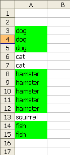
I have a report listing sales orders, or more specifically, each line of a sales order. I want to alternately color each sales order so there’s a nice visual separation, but I don’t know how many lines each sales order will have. If my sales order numbers were animal names and I was color blind, it might look like this:

The conditional formatting for this color banding is shown below.

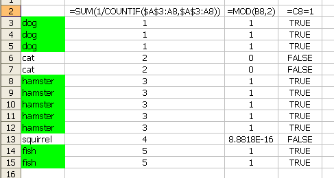
The formula uses a David Hagar formula from Chip Pearson’s site to determine the number of unique entries in the list. This has the effect of numbering the unique entries. The MOD function determines if it’s even or odd and only odd entries are formatted.
This shows how the formula evaluates out. All the formulas in the worksheet are entered as array formulas (Control+Shift+Enter), but the CF formula is entered normally. The formulas shown are from line 8, if you couldn’t tell.

Pretty clever, Dick. The only problem is using the absolute reference. If you insert a new row above, or if you move the range, the formula no longer works. I tried to figure out a way around this, but I gave up after 30 minutes. I’m sure someone will come up with a solution.
I agree John (about the problem, not that I’m clever). Another problem is the imprecision in the MOD function, like in the squirrel example. While it worked there, it could have easily not worked somewhere else. If anyone uses this, be sure to wrap your MOD function in a ROUND function, e.g.
This is repeat to work around the problem with a less than sign. Hopefully, Dick will delete the first one.
Dick:
Slick.
And, did you forget our date?
John:
Define 2 names:
DataRng=OFFSET(Sheet1!$H$5,0,0,COUNTA(Sheet1!$H:$H),1)
FirstCell=Sheet1!$H$5
Now, use the c.f.
=ABS(MOD(SUM(1/COUNTIF(FirstCell:INDEX(DataRng,ROW()-ROW(FirstCell)+1),FirstCell:INDEX(DataRng,ROW()-ROW(FirstCell)+1))),2)-1)<0.000001
The above is OK for inserting rows but not for moving the range to another column. Unless, of course, one moves the entire column. The problem with moving the range to another column is that the H:H reference in the DataRng is not updated.
Delete done. I didn’t forget our date, I was there at 11AM CDT. I figured you got busy. Did I get the time wrong?
One can solve the problem of moving the range with the following change to the names:
FirstCell=Sheet1!$H$5
DataRng=OFFSET(FirstCell,0,0,COUNTA(INDEX(Sheet1!$1:$65536,,COLUMN(FirstCell))),1)
Also — and this in no way is meant to take away from Dick’s really creative solution — if one uses an extra column the process can be significantly simplified. Suppose the data are in H starting with H2. Then, in I2 enter the formula =IF(H2=H1,I1,MOD(I1+1,2)) Now, the c.f. for H2 would be =$I2=1
The I2 formula is one I have used on many occasions. It — or a variant — is a simple way to identify each change in values in a column.
And, 11AM CDT is noon EDT, not 10AM EDT. We should try again using the time in your time zone. I’ll adjust to whatever zone I am in that day. {grin} I’ll use your gmail account for a follow up message.
Hello,
try for cell A3:
=MOD(SUM(1/COUNTIF($A$3:$A3,$A$3:$A3)),2)>0.5
Example in German language but with demonstration:
http://www.online-excel.de/excel/singsel.php?f=75#s29
——————-
Or this:
=MOD(SUM(N($A$1:$A2$A$2:$A3)),2)
Example in German language but with demonstration:
http://www.excelformeln.de/tips.html?welcher=70
Both are for sorted lists.
Regards,
Beate
Sorry,
the 2nd formula is scrambled. Another trial, otherwise pls refer to link:
=MOD(SUM(N($A$1:$A2$A$2:$A3)),2)
Regards,
Beate
I did this a while ago. This requires more steps but seems to require less processing power.
1. Put a 1 in G3.
2. In G4 insert the formula below and copy down:
=(A4A3)*(G31)+(A4=A3)*G3
3. Highlight row 4 and under cond. formatting use:
=$G4=0
4. Copy the cond. formatting down.
Jason
Sorry, that should be NOT EQUAL between A4 and A3 and G3 NOT EQUAL 1, not G31.
If you are allowed to refer to another cell, i.e. apply conditional formatting if other cell =TRUE then this works: =OR(AND(B2=TRUE,A3=A2),AND(B2=FALSE,A3 ‘not equal to’ A2)). ‘B2’ is one cell above the ‘test list’; the ‘test cell’ copied down, in this case is in column B.
Personally I have an irrational dislike to the MOD function :)
Andrew
A bit off topic, but I had a need to have every other row’s background shaded with color (and the others white). It is similar to this post. I used it to make a large spreadsheet easier to read. At first I tried copying two rows by right-clicking the fill handle and choosing “fill formats only”. However any time I hid, deleted, or inserted a row, I had to re-do. So I used this conditional format: =MOD(Subtotal(103, $A$2:$A2)+1,2) where my region starts with A2. Note that column A can’t be blank.
This maintains the formatting with hides, unhides, and deletions. If you simply copy an existing row and Insert Copied Cells, the formatting is maintained.
Hopefully this will help someone, Enjoy!
I see a lot of difficult statements, just think simple.
I have 2 columns:
a b
one 1
one 1
one 1
two 0
two 0
two 0
three 1
three 1
four 0
First I sort column A. Then I insert my temp-column, B. In the first cel of B i put the value ‘1’. Then in B2 i put the formula: =ALS(A2A1;ALS(A1=1;1;0);B1). I copy the formula to the bottom. Then I select the complete A column. I use conditional formatting with the following formula: =$B1=1. If this is true I highlight the cel.
Simpel, and works perfect!
The formula in my last post is not displayed correctly, i don’t know why. It reads like =IF(A2 NOT EQUALS A1;IF(A1=1;1;0);B1). The NOT EQUALS signs where not displayed!
To Jason B — about formating every second row with different colors:
It would be easier to use just MOD(ROW(),2)=1 instead, which would give you exactly the same result without having reference to your area. If you would like, then you can even use AND(A1?”,MOD(ROW(),2)=1)=TRUE in column A to have formating only in the cells, that have some content inside — so the formating automatically expands, once you are filling your table :)