I’ve been recently using the great guides from (what used to be) SpreadsheetStyle.com.
I’m a real fan of the 3 crayon rule.
I see other Excel users with a rainbow of colours on their sheets. I ask them “why all the colours?” and they reply “see, the red cells are errors and the green cells do this and the grey cells do that and… well… noone else uses this spreadsheet so only I need to know what the colours mean”.
Only they need to know! Until they get another job. Why were those cells highlighted again?
Here is where it’s nice to have a worksheet legend:
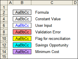
Leaving some cells dedicated to a Legend can be a little cluttered, so here is a way to put the legend in as a cell comment.
I used an Excel add-in for exporting my range as a picture. That saves me from writing a macro to do the same.
There are a few add-ins which can do this. I use Andy Pope’s Graphics Exporter
Highlight your range, say, A1:D15
From the Tools menu, select Graphics Exporter.
Note the Output folder and click Export.
Click a blank cell. From the Insert menu, select Comment.
Delete the text in the new comment box.
Notice how the border style is diagonal lines. Click it and it changes to a dotted border style.
From the Format menu, select Comment.
The Format Comment window appears
From the Colors and Lines tab, click the Fill Color dropdown box and select Fill Effects.
The Fill Effects window appears
From the Picture tab, click Select Picture.
Browse to where you exported that picture, select the file and click Insert.
Tick the ‘Lock picture aspect ratio’ box.
Click OK then OK again.
Depending on your comment box defaults, you’ve probably got what appears to be a tiny picture in the comment box.
You can resize it to whatever dimensions you like, but here is a tip to get your comment box matching the dimensions of your picture.
(This will only work if you ticked the ‘Lock picture aspect ratio’ as described earlier)
Resize the comment box so that it is quite tall.
Nudge the width wider and wider until it starts scaling the picture.
The point where it starts scaling the picture is where both the picture and comment box dimensions match.
Then, with the Shift key held down, drag the bottom-right handle so it resizes both height and width at the same time.
(The Shift key maintains the width/height ratio)
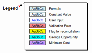
In the end you should end up with something like this:
I assume this is possible in an newer version than 9.0 a.k.a. Excel 2000, since I can’t find that picture tab but the Colors and Lines tab does exist?
Greetings,
Peter
Peter,
I run Excel 2003, so I can’t check to be sure… I thought I remembered the feature being there for 97.
Could you please double check something for me?
On the ‘Colors and Lines’ tab, there are 3 sections: Fill, Line and Arrows.
In the Fill section there is a dropdown box for choosing a fill ‘Color’.
Click the ‘Color’ dropdown box and tell me whether there is a selection available called ‘Fill Effects’?
Cheers,
Rob
Peter,
The Picture tab is not at that level you need to go a little deeper.
Click the Color dropdown, you should see a matrix of colours and 2 further menu options, More colors and Fill effects. Click the fill effects and now you should have the dialog with the picture tab.
Neat trick by the way Rob.
Pretty good idea Rob.
You’re absolutely right, Rob. There such a thing as Fill effects at he bottom with another dialog with the tab mentioned. Thanks for pointing that out to me.
Dat krijg je nou als je niet verder kijkt dan je neus lang is. (This last one is for the Dutch readers of this blog among us.)
Peter
See also Debra’s site
http://www.contextures.com/xlcomments02.html#Picture